Top-Down Programming Meets the Game of Life

The first function in the Game of Life hierarchy

To implement the Game of Life, we will apply top-down programming to write a concise function PlayGameOfLife(). This function will take as input the initial configuration of the board, initialBoard, as well as the number of generations, numGens. To play the Game of Life over numGens generations, we will repeatedly call a subroutine UpdateBoard() to update a given board into its next generation.

PlayGameOfLife(initialBoard, numGens)
    boards ← array of numGens + 1 game boards
    boards[0] ← initialBoard
    for every integer i from 1 to numGens
        boards[i] ← UpdateBoard(boards[i–1])
    return boards

Note that we can write PlayGameOfLife() without even specifying what the type of the Game of Life “game board” should be. But in order to write UpdateBoard(), we should be more precise about this type.

A bit about arrays

Since the beginning of the course, we have used arrays to store multiple values in the form of a table. Although we have thus far only worked with one-dimensional arrays (i.e., single rows of values), arrays can also be two- or multi-dimensional. To implement the Game of Life, we will use a two-dimensional array of boolean variables in which true corresponds to “alive” and false corresponds to “dead”.

false	false	false	false	false
false	false	true	true	false
false	true	true	false	false
false	false	true	false	false
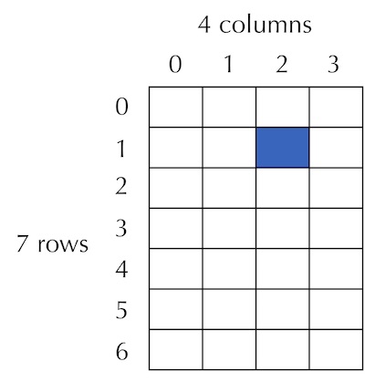
false	false	false	false	false

Before continuing with implementing UpdateBoard(), we will make a few remarks about working with two-dimensional arrays. Given a two-dimensional array a, the notation a[r] typically refers to all of the elements in row r of a, and a[r][c] refers to the single element in row r and column c. Extending the paradigm of 0-based indexing, in an array with n rows and m columns, the rows are indexed from 0 to n-1, and the columns are indexed from 0 to m-1. Accordingly, the highlighted element in the figure below would be denoted a[1][2].

To access all the rows of an array a with n rows and c columns, we would apply the following pseudocode.

for every integer r between 0 and n-1
    access a[r]

We will think of the row a[r] as a one-dimensional array. To access all the elements of row a[r], we will let an integer c range from 0 to m-1 and access a[r][c]. This provides us with an insight into how to access all of the elements of a: we range over every row r, and then for each value of r, we range over every column value c.

for every integer r between 0 and n-1
    for every integer c between 0 and m-1
        access a[r][c]

Updating a Game of Life board

Now that we know how to range over the elements of a two-dimensional array, we can write UpdateBoard(). In keeping with top-down design, just as we play the Game of Life one generation at a time, we update a game board one cell at a time. That is, we will rely on a pseudocode function UpdateCell() that takes as input the current Game of Life board currentBoard as well as row and column integers r and c; this function returns true or false corresponding to whether the cell currentBoard[r][c] will be respectively alive or dead according to the Game of Life rules in the next generation.

The pseudocode below also calls an InitializeBoard() subroutine that takes integers numRows and numCols as input and returns a two-dimensional game board in which all values are set to false. (We will write this function when implementing the Game of Life in a specific language in this chapter’s code alongs.)

UpdateBoard(currentBoard)
    numRows ← CountRows(currentBoard)
    numCols ← CountCols(currentBoard)
    newBoard ← InitializeBoard(numRows, numCols)
    for every integer r between 0 and numRows – 1
        for every integer c between 0 and numCols – 1
            newBoard[r][c] ← UpdateCell(currentBoard, r, c)
    return newBoard

You may be concerned that we have not yet handled the most important details of implementing the Game of Life. How should we apply the rules of the game? How should we handle cells on the boundary of the board? Delaying such details tends to make new programmers anxious; should we not focus on the trickiest aspects of our code first? Yet we will see that our work often winds up being easier than anticipated if we delay challenging aspects of an implementation to lower levels of the function hierarchy.

We now will write UpdateCell(), applying the rules of the Game of Life in UpdateCell() by calling a subroutine CountLiveNeighbors(). This function takes as input currentBoard as well as r and c, and it returns the number of live neighbors in the Moore neighborhood of currentBoard[r][c]. CountLiveNeighbors() will also allow us to handle cells at the edge of the board, since if a neighboring cell is not on the board, then we will by default consider it to be dead.

UpdateCell(currentBoard, r, c)
    numNeighbors ← CountLiveNeighbors(currentBoard, r, c)
    if currentBoard[r][c] = true (current cell is alive)
        if numNeighbors = 2 or numNeighbors = 3 (propagation)
            return true
        else (no mates/overpopulation)
            return false
    else (current cell is dead)
        if numNeighbors = 3 (zombie!)
            return true
        else (rest in peace)
            return false

Counting live cells in a neighborhood

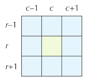
We now turn to implementing CountLiveNeighbors(). As shown in the figure below, the Moore neighborhood of a cell in row r and column c contains cells between rows r − 1 and r + 1 and between columns c − 1 and c + 1.

To range over the cells in a Moore neighborhood, we should apply the same idea that we used when ranging over an entire array: range over the row indices using a for loop, and within this for loop range over the column indices. This idea brings us to the following implementation of CountLiveNeighbors().

CountLiveNeighbors(currentBoard, r, c)
    count ← 0
    for every integer i between r–1 and r+1
        for every integer j between c–1 and c+1
            if currentBoard[i][j] = true
                count ← count + 1
    return count

Consider the two for loops in CountLiveNeighbors() as this function is currently written.

    for every integer i between r – 1 and r + 1
        for every integer j between c – 1 and c + 1

At some point in these loops, i will be equal to r and j will be equal to c. Yet this is the cell currentBoard[r][c] under consideration! To avoid including a cell in its own Moore neighborhood, we should only consider currentBoard[i][j] in CountLiveNeighbors() if this cell does not coincide with currentBoard[r][c]; that is, if i ≠ r or j ≠ c. This produces the updated CountLiveNeighbors() function shown below.

CountLiveNeighbors(currentBoard, r, c)
    count ← 0
    for every integer i between r – 1 and r + 1
        for every integer j between c – 1 and c + 1
            if i≠r or j≠c
                if currentBoard[i][j] = true
                    count ← count + 1
    return count

You are now allowed to be concerned that we have not handled the boundary of the board. For example, consider what would happen if we called CountLiveNeighbors() if r is equal to zero. Because we range i between r-1 and r+1, i will start equal to -1, and we will be trying to access cells of the form currentBoard[-1][c], which don’t exist! As a result, our program will encounter an error. We will encounter similar problems if c is equal to 0 or if r or c is equal to their maximum possible values.

We will be able to patch the hole in our pseudocode by adding a subroutine to check whether currentBoard[i][j] is contained within the boundaries of the board. The following function called InField() takes as input currentBoard along with row and column indices i and j; it returns false if the cell currentBoard[i][j] lies outside of the board and true otherwise.

InField(currentBoard, i, j)
    numRows ← CountRows(currentBoard)
    numCols ← CountCols(currentBoard)
    if i < 0 or i > numRows-1 or j < 0 or j > numCols-1
        return false
    else
        return true

Now that we have written InField(), we will add it as a subroutine call to CountLiveNeighbors() to ensure that  currentBoard[i][j] is within the board in addition to our previous test that i ≠ r or j ≠ c. To join these two tests, we can use the and keyword.

CountLiveNeighbors(currentBoard, r, c)
    count ← 0
    for every integer i between r – 1 and r + 1
        for every integer j between c – 1 and c + 1
            if (i≠r or j≠c) and InField(currentBoard, i, j) = true
                if currentBoard[i][j] = true
                    count ← count + 1
    return count

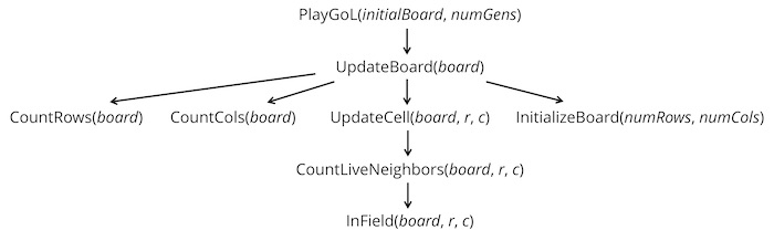
And just like that, we have solved the Game of Life problem, whose complete function hierarchy is shown in the figure below. Soon we will get to apply this hierarchy in the context of a programming language and code the Game of Life!

Printing Game of Life boards

Top-down design is powerful because it leverages the principle of modularity, in which we write many functions, each with a single specific purpose. An important strength of code modularity is the division between data generation and data visualization. Beginner programmers sometimes conflate these two concepts, trying to visualize data at the same time as it is being generated. In this case, we have thus far worked on generating the data corresponding to a collection of Game of Life boards, and now we can turn to visualizing the Game of Life over multiple generations as a separate process.

We will leave more sophisticated image rendering to individual programming languages, but we will point out that (as you will know from following our code alongs) programming languages all have a built-in Print() function that prints an input string to the console. To print a collection of Game of Life boards to the console one at a time, we could proceed top-down again, dividing the task into many calls to a PrintBoard() subroutine that prints a single board.

PrintBoards(boards)
    for every integer i from 0 to len(boards) - 1
        PrintBoard(boards[i])

One way to write PrintBoard() would be to range over all of the rows of the input board, and then range over all the columns of the board, printing one value at a time. At the end of each line, we need to print a new line.

PrintBoard(board)
    for every integer i from 0 to CountRows(board) - 1
        for every integer j from 0 to CountCols(board) - 1
            Print(board[i][j])
        Print(new line)

Yet we have adopted a top-down, modular mindset, and such a framework means that we can avoid nested loops by instead calling a subroutine. In this case, we will still range over the rows of the board, but we will then print each row by calling a separate PrintRow() subroutine that ranges over every cell in a given row (a one-dimensional array) and prints that cell. We will print a blank line at the end of PrintRow(), which brings us to the following shortened PrintBoard() function along with PrintRow().

PrintBoard(board)
    for every integer i from 0 to CountRows(board) - 1
        PrintRow(board[i])

PrintRow(row)
    for every integer j from 0 to len(row) - 1
        PrintCell(row[j])
    Print(new line)

Finally, we must write a function to print a single boolean value, which simply tests whether the cell is true or false and prints a black square or white square accordingly.

PrintCell(value)
    if value = true
        Print("⬛")
    else 
        Print("⬜")

We will use these functions as a starting point for building a more sophisticated visualization to produce an animated GIF of the Game of Life in a code along. For now, we will return to von Neumann’s original goal of finding a self-replicating cellular automaton. Does such an automaton exist?