A short history of self-replicating automata
In 1952, almost two decades before the discovery of the Gosper gun for the Game of Life, von Neumann discovered a self-replicating cellular automaton. Here is famed biologist Sydney Brenner talking about the work of von Neumann, who not only included a specification of a self-replicating automata, but also theorized about the fundamentals of what properties self replicating systems would have. Von Neumann had no idea that several thousand miles away at the same time, Watson, Crick, Franklin, and Wilkins were uncovering the self-replicating system that serves as the genetic foundation of all living things: DNA.
And yet the Game of Life enjoys widespread popularity among the nerd élite, while von Neumann’s work on self replication is still largely uncelebrated. How could this be?
Part of the reason for its popularity is that the Game of Life exhibits an enormous amount of complex behavior from five very simple rules that can be taught to a child and while only allowing two states for cells (alive and dead). In contrast, von Neumann’s self-replicating cellular automaton had 29 states and a mind-boggling 130,622 cells. This automaton hardly meets von Neumann’s own desire for a self-replicator that is simply defined; can we find a smaller pattern with fewer states?
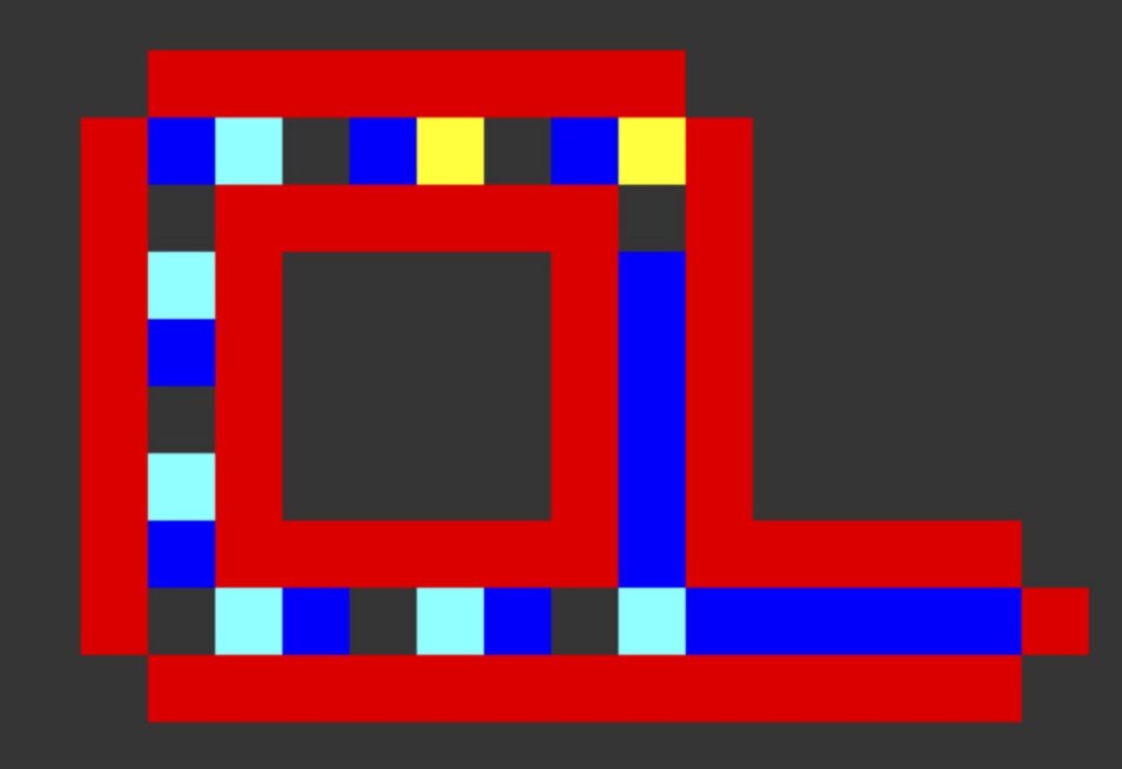
This question remained open for over three decades. In the meantime, Edgar Codd produced a self-replicating cellular automaton with only eight states in 1968, but the pattern exhibiting the self-replication had nearly 300 million cells. Only in 1984 did Christopher Langton manage to find an 8-state self-replicating cellular automaton with only 86 cells that has come to be called Langton’s loop, shown in the figure below.
Formalizing the rules of an automaton
In what follows, we wish to implement Langton’s loop and visualize its self-replication for ourselves. But it seems silly to start the whole process over. Instead of treating Langton’s loop as a separate case to the Game of Life, why don’t we devise an algorithm that implements any two-dimensional cellular automaton? We can state this goal as the following computational problem; solving this problem will illustrate another paradigm of programming, which is generalizing an existing solution to a specific problem to solve a broader problem.
Cellular Automaton Problem
Input: An initial configuration of a cellular automaton initialBoard, an integer numGens, and a collection of rules rules for the automaton.
Output: All numGens + 1 configurations of the automaton over numGens generations starting with initialBoard and following the rules indicated in rules.
To make the Cellular Automaton Problem more concrete, we need to do two things. First, as we transition from two states to an arbitrary number of states, using boolean variables in our array will no longer suffice. To address this issue, we will represent an arbitrary automaton as a two-dimensional array of integers.
Second, we need a clear and concise way of representing the rules of a cellular automaton.
STOP: How could we succinctly summarize the rules of the Game of Life? What about the rules of an arbitrary cellular automaton?
One way to succinctly represent the rules of a two-state automaton like the Game of Life would be with what is known as BySx format. In this format, y is the number of live neighbors needed for “birth” (i.e., for a dead cell to become alive), and x is the number of live neighbors for “survival” (i.e., for an alive cell to remain alive). The BySx format for the Game of Life is B3S23; if we know that birth can only happen with three live neighbors, and that survival can only happen with two or three live neighbors, then the conditions for a cell dying or remaining dead can be inferred immediately.
Yet unfortunately BySx format will not work for a general cellular automaton with more than two states, not to mention rules that not only count the number of cells of a certain type in a cell’s neighborhood, but that also account for the configuration of these cells. For example, a two-state automaton might update a given live cell with two live neighbors to be alive or dead depending on the configuration of those two neighbors, as illustrated in the figure below.
STOP: How can we represent each of the two rules in the figure below succinctly?
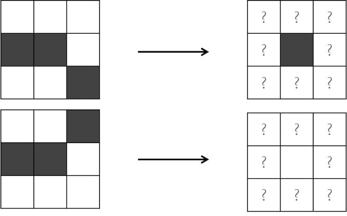
To represent a cell and its Moore neighborhood, we will use a neighborhood string containing nine symbols. The first character encodes the state of the cell under consideration, and the next eight characters encode the states of the neighbors of the cell. In this chapter, we will read the neighbors clockwise from top left. For example, using “0” to denote “dead” and “1” to denote “alive”, the two neighborhoods on the left side of the figure above would be represented as “100001001” and “100100001”.
Note: When converting a Moore neighborhood to a string, we could start at a different neighbor or proceed counterclockwise, as long as we were always consistent in this choice.
Exercise: Draw the nine cells corresponding to the neighborhood string“011100110”.
We can now represent a cellular automaton’s rules as a rule map whose keys are neighborhood strings and whose values are integer, where we associate each neighborhood string to the value of the cell in the next generation according to the neighborhood. For example, we could represent the two rules in the figure above with a map containing “100001001”:1 and “100100001”:0.
Exercise: How many rules does a generalized two-state cellular automaton have?
To answer the preceding exercise, both a cell and each of its neighbors can be either alive or dead, so that the neighborhood strings will be every possible string of zeroes and ones of length 9. As a result, a cellular automaton will need 29 = 512 different strings to represent all possible rules.
Exercise: How many different possible two-state cellular automata “games” are there? How many different possible k-state cellular automata “games” are there?
von Neumann neighborhoods
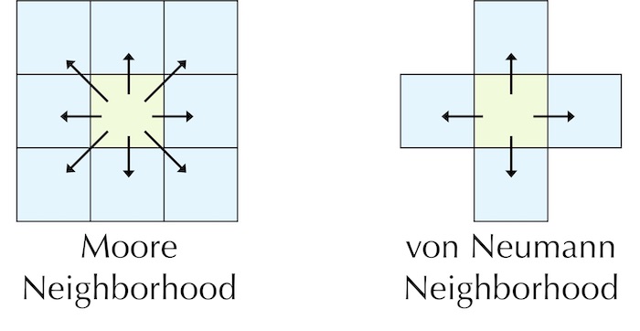
We have moved our target from programming a single cellular automaton to programming any of a cosmically large number of automata. But before we undertake this goal, we will make the problem even more general by introducing a new neighborhood used by many automata, including Langton’s loop and the automaton that von Neumann introduced. In the von Neumann neighborhood of a cell, we only consider a cell’s four adjacent cells (see figure below).
We should also adapt our rule strings to accommodate cellular automata with von Neumann neighborhoods. The neighborhood string of a cell will consist of the cell’s state in addition to those of its four neighbors; our convention is to read the neighbors clockwise, starting with the top neighbor. As a result, the two rules illustrated in the figure below are represented by “10001”:1 and “01110”:0.
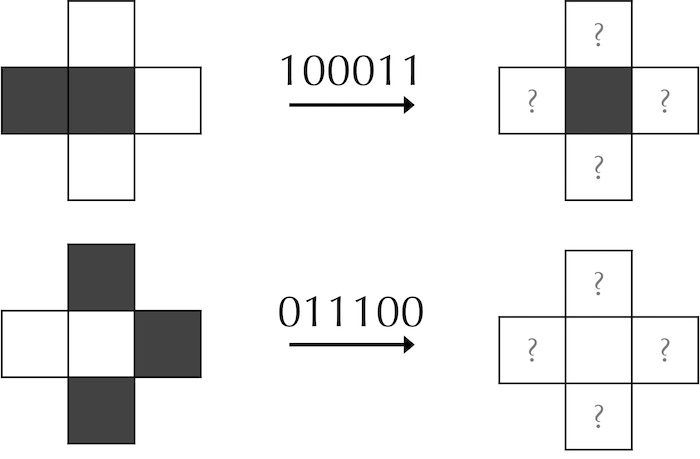
“100011”:1 and “011100”:0.Exercise: How many different possible k-state cellular automata are there if we use a von Neumann neighborhood?
Now that we have found a way to represent the rules of an arbitrary cellular automaton, we can improve our statement of the Cellular Automaton Problem.
Cellular Automaton Problem
Input: An initial configuration of a cellular automaton initialBoard, an integer numGens, a string neighborhoodType indicating the type of neighborhood considered, and a map of strings to integers rules encoding the rules of the automaton.
Output: All numGens + 1 configurations of this board over numGens generations starting with initialBoard, following the rules indicated in ruleStrings and using the indicated neighborhood type neighborhood.
Note: Technically, we will only be able to represent cellular automata with ten states or fewer, since we will only be able to use the digits 0 to 9 to represent states. However, for the purposes of this chapter, this assumption will suffice, especially if you have completed our challenge exercise on counting the number of possible cellular automata with ten states. 😉
Implementing a general cellular automaton
Writing the highest level function
We need to generalize our function hierarchy for PlayGoL() to a function hierarchy for a function PlayAutomaton() solving the Cellular Automaton Problem. This function will need to take two additional parameters: neighborhoodType is a string that will either be equal to “vonNeumann” or “Moore”, and rules is a map of strings to integers containing the rules for the automaton. Using PlayGameOfLife() as a model, we obtain the following function, where we pass neighborhoodType and ruleStrings to a generalized UpdateBoard() subroutine.
PlayAutomaton(initialBoard, numGens, neighborhoodType, rules)
    boards ← array of numGens+1 game boards
    boards[0] ← initialBoard
    for every integer i from 1 to numGens
        boards[i] ← UpdateBoard(boards[i – 1], neighborhoodType, rules)
    return boards
Updating one generation of an automaton
As for UpdateBoard(), we will apply the same idea, passing both of the new parameters down into an appropriate subroutine and delaying details for as long as we can.
UpdateBoard(currentBoard, neighborhoodType, rules)
    numRows ← CountRows(currentBoard)
    numCols ← CountColumns(currentBoard)
    newBoard ← InitializeBoard(numRows, numCols)
    for every integer r between 0 and numRows – 1
        for every integer c between 0 and numCols – 1
            newBoard[r][c] ← UpdateCell(currentBoard, r, c, neighborhoodType, rules)
    return newBoard
Updating one cell
To update a single cell, we will need to look for the key in rules that is equal to the neighborhood string of the given cell, and then return the value associated with this string in rules. As a result, UpdateCell() will be a very short function if we assume a subroutine NeighborhoodToString() that takes as input a game board currentBoard, integers r and c, and neighborhoodType, and that returns the neighborhood string of currentBoard[r][c].
UpdateCell(currentBoard, r, c, neighborhoodType, rules)
    neighborhood ← NeighborhoodToString(currentBoard, r, c, neighborhoodType)
    return rules[neighborhood]
Generating the neighborhood of a cell as a string
We are now at the bottom of our function hierarchy and are ready to implement NeighborhoodToString(). As is often the case at the bottom of the function hierarchy, this function gets pretty ugly, but at least it gives us the opportunity to practice our skills with indexing a two-dimensional array.
NeighborhoodToString(currentBoard, r, c, neighborhoodType)
    neighborhood ← "" + currentBoard[r][c]
    if neighborhoodType = "Moore"
        ruleString ← ruleString + currentBoard[r-1][c-1] + currentBoard[r-1][c] + currentBoard[r-1][c+1] + currentBoard[r][c+1] + currentBoard[r+1][c+1] + currentBoard[r+1][c] + currentBoard[r+1][c-1] + currentBoard[r][c-1]
    else if neighborhoodType = "vonNeumann"
        ruleString ← ruleString + currentBoard[r-1][c] + currentBoard[r][c+1] +  currentBoard[r+1][c] + currentBoard[r][c-1]
    return neighborhood
STOP: This function has a bug. What is it?
As when implementing the Game of Life, the bottom of our function hierarchy for PlayAutomaton() is the time for us to be concerned about cells on the boundary of the board. In particular, with the current implementation of NeighborhoodToString(), any cell on an outside column of the board would have one of its neighbors outside of the range of the board.
We now need to make a design decision with our automata. We could expand our collection of neighborhood strings to handle cells on the outside of the board. Yet for most automata, defining all those rules will become tricky; in fact, Langton did not even consider rules for the exterior of the board when designing his self-replicating cellular automaton. Instead, we will assume that any cells falling outside the board have state equal to 0, which is the default “dead” state used in the background of all cellular automata (and shown in gray in the Langton loop figure).
To implement this idea, we will use a two-dimensional array neighbors for which each row contains two values: the x- and y-coordinates of one of the neighbors of currentBoard[r][c]. For example, these ordered pairs for the von Neumann neighborhood are [[r-1, c], [r, c+1], [r+1, c], [r, c-1]]. We can then access the elements of a cell’s neighborhood by ranging over the rows of offsets and adding each row’s x-coordinate (its first element) to r and each row’s y-coordinate (its second element) to c.
Each time we identify the indices of a cell, we check whether this cell is on the board using our old friend InField(). If so, we append this cell’s value to the growing neighborhood string; if not, we append 0 to neighborhood.
These ideas bring us the following revised implementation of NeighborhoodToString(). More importantly, we have now implemented an arbitrary cellular automaton and are ready to convert our work into code!
NeighborhoodToString(currentBoard, r, c, neighborhoodType)
    neighborhood ← "" + currentBoard[r][c]
    offsets ← empty two-dimensional array
    if neighborhoodType = "Moore"
        neighbors ← [[r-1, c-1], [r-1, c], [r-1, c+1], [r, c+1], [r+1, c+1], [r+1, c], [r+1, c-1], [r, c-1]]
    else if neighborhoodType = "vonNeumann"
        offsets ← [[r-1, c], [r, c+1], [r+1, c], [r, c-1]]
    for i ← 0 to len(offsets) - 1
        x ← offsets[i][0]
        y ← offsets[i][1]
        if InField(currentBoard, r+x, c+y)
            neighborhood ← neighborhood + currentBoard[r][c]
        else
            neighborhood ← neighborhood + "0"
    return neighborhood
Exercise: We could also handle boundary cells by having neighborhoods “wrap around” the sides of the board. For example, cells on the bottom of the board will have cell(s) in the top row as their neighbor. How could we reviseNeighborhoodToString()to handle this situation?
Design top down, debug bottom up
We will pause to make the point that it would be easy to incorporate bugs into a function like NeighborhoodToString()because of a typo. Imagine, for example, if we were to replace one of the occurrences of -1 in the declaration of offsets with a 1. An irony of top-down programming is that it is probably more difficult to incorporate a bug into a function like PlayAutomaton() that is high up in a function hierarchy because it passes complicated details to subroutines of subroutines. And a benefit of top-down programming is due to the simple fact that it is easier to test and debug a short function than a long one.
In this case, we could test NeighborhoodToString() by giving this function a few small boards with values on edges and corners to make sure that the function works, which is exactly how our autograder works.
Moreover, when testing any top-down code, you should start by testing functions like InField() that are at the bottom of the function hierarchy because they do not call subroutines, so any bugs will be confined to these functions. Once we feel good about our implementation of InField(), we can next consider NeighborhoodToString() as we work our way up the function hierarchy. In short, whereas we often plan our programs top-down, we often debug and test our code bottom-up.
Langton’s Loops and artificial life
We hope that you will follow our code alongs, but we will provide a spoiler in the form of a video of Langton’s loops below. Please take a moment to reflect that this simple pattern took 30 years to discover after cellular automata were first discovered. Notice also that the cells not only self-replicate, but after a period of time, they enter a “death” state in which they no longer have cells that change state. In this sense, they mimic life itself.
One of the enduring qualities of Langton’s loops is how lifelike they seem. We would not be unreasonable to notice that the loop itself vaguely resembles a cell, or that its three-cell wide outer shell is reminiscent of a biological molecule like DNA that has a two-sided exterior with information represented inside the molecule.
You likely have never heard of artificial life because after some early excitement, the field largely failed to produce any substantive research results and mostly flamed out in the 1990s. Artificial life offers an excellent example of what can happen to a perfectly reasonable area of scientific interest when it becomes oversold. Today we have the field of “artificial intelligence”, which was often ridiculed for years only now to demonstrate immense hope and progress.
Finally, while philosophizing, we would return to the start of this chapter and the Fermi paradox. Perhaps we have not seen self-replicating space probes not because alien life isn’t out there, but because other civilizations find self-replicating robots just as difficult to build as we do. If it took 30 years just to discover a simple self-replicating cellular automaton, maybe the fact that the trillions of cells in your body go about their business of self-replication every day is something of such depth and elegance that we take it for granted.
Or maybe the resolution to the Fermi paradox is something much simpler. Maybe our lust for exploration makes us a peculiar species. Maybe the aliens know how to build von Neumann probes, but they are too busy enjoying existence to be bothered.
It’s time to code
We have learned a great deal about top-down programming and cellular automata, and now you are ready to apply this knowledge to a specific programming language and build the Game of Life and Langton loops. Click “next lesson” to join us!