Simulating a Presidential Election

Planning the simulation of multiple elections

We can learn from our work with computing the house edge of craps that a natural way to run many election simulations is to pass the heavy lifting to a function that simulates a single election. The pseudocode below for a SimulateMultipleElections() function does just this.

In practice, different polls have different margin of errors, reflecting variables like number of respondents or historical reliability of the poll. However, we will assume that the margin of error is a fixed parameter called marginOfError. We will use this parameter to incorporate random bounce into our simulations. If this parameter is 0.06, then we are approximately 95% confident that our state poll is accurate within 6% in either direction. For example, if candidate 1’s polling percentage in California is 64%, then we are 95% sure that the true percentage of voters supporting candidate 1 is between 58% and 70%.

We will also not specify yet how the polling data will be represented; for the time being, we will just call these data pollingData, a parameter that we will pass along with marginOfError to the SimulateOneElection() subroutine, which returns the number of Electoral College votes each candidate receives in a single simulated election.

We will now present SimulateMultipleElections(), which calls SimulateOneElection() a total of numTrials times, keeping track of the number of wins each candidate accumulates (as well as the number of ties). It then divides each win count by the total number of trials to obtain estimated “probabilities” of each candidate winning, along with the estimated probability of a tie.

SimulateMultipleElections(pollingData, numTrials, marginOfError)
    winCount1 ← 0
    winCount2 ← 0
    tieCount ← 0
    for numTrials total trials
        votes1,votes2 ← SimulateElection(pollingData, marginOfError)
        if votes1 > votes2
            winCount1 ← winCount1 + 1
        else if collegeVotes2 > collegeVotes1
            winCount2 ← winCount2 + 1
        else (tie!)
            tieCount ← tieCount + 1
    probability1 ← winCount1/numTrials
    probability2 ← winCount2/numTrials
    probabilityTie ← tieCount/numTrials
    return probability1, probability2, probabilityTie

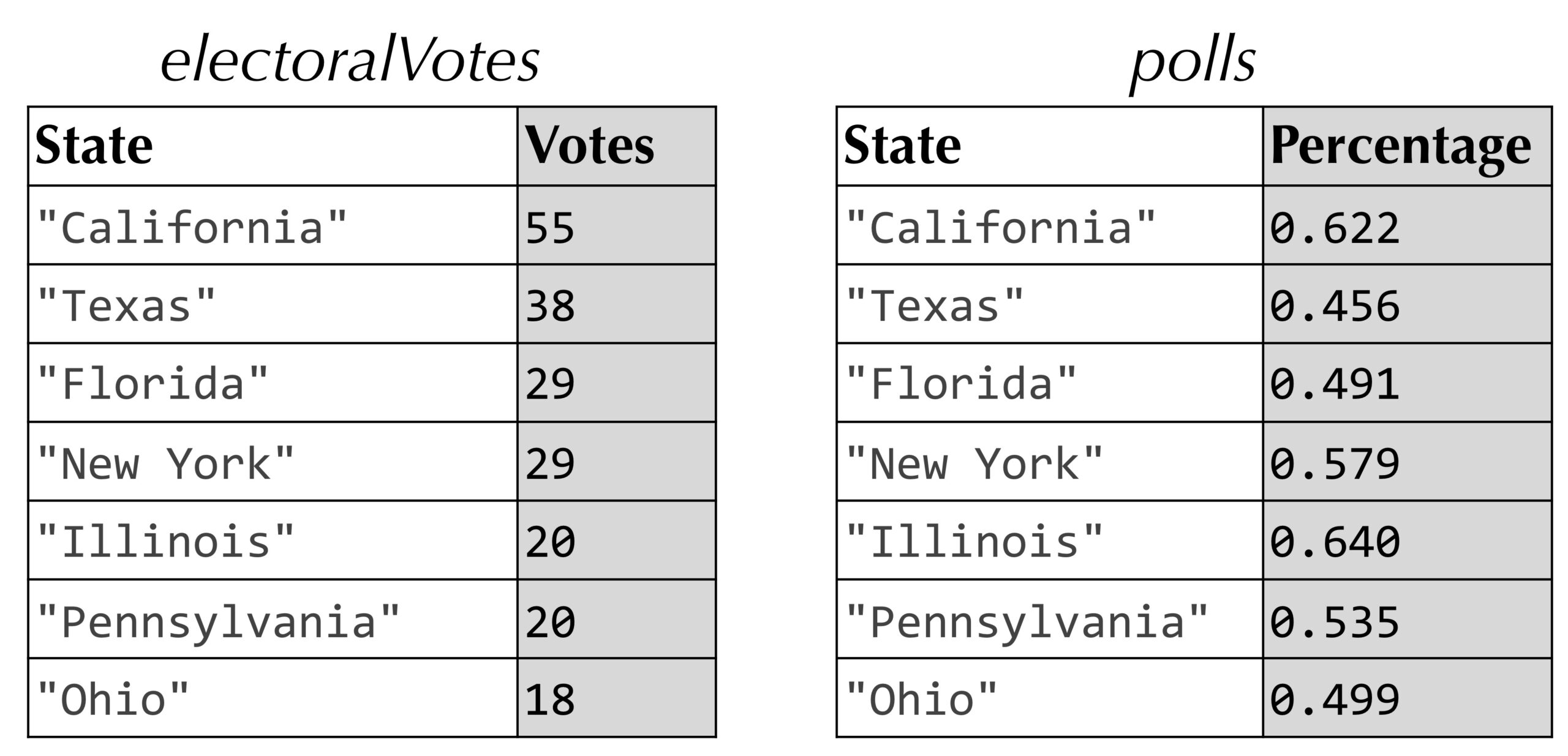
A natural way to represent pollingData is as two maps (see figure below). An electoralVotes map associates state name keys with the (positive) integer storing the number of votes for that state. A polls map associates state name keys with the percentage at which candidate 1 is polling in that state.

Simulating a single election

To simulate a single election, we need to use these polling data along with marginOfError to produce a randomly adjusted polling percentage for each state. If this adjusted percentage is greater than or equal to 50%, then we assume that candidate 1 wins the state (a tie will be extremely unlikely). We will return to discuss the details of this adjustment soon; for now, we will call the subroutine that achieves this objective AddNoise(). The SimulateOneElection() function could return which candidate wins (or if there was a tie), but we will have this function return the number of electoral votes that each candidate wins in the simulated election.

SimulateOneElection(polls, electoralVotes, marginOfError)
    votes1 ← 0
    votes2 ← 0
    for every key state in polls
        poll ← candidate 1's polling percentage
        adjustedPoll ← AddNoise(poll, marginOfError)
        if adjustedPoll ≥ 0.5 (candidate 1 wins state)
            votes1 ← votes1 + electoralVotes[state]
        else (candidate 2 wins state)
            votes2 ← votes2 + electoralVotes[state]
    return votes1, votes2

As with our work with craps, we see that the randomization is lurking within a subroutine, which in this case is the AddNoise() function.

Adding noise to each state’s polling value

Unlike our previous work, using RandInt() or RandIntn() is unnatural because we need to generate a random decimal number x that we will be adding to candidate 1’s polling percentage. One idea is to generating a noise value between -marginOfError and marginOfError by first generating a pseudorandom decimal number between -1 and 1, and then multiplying the resulting value by marginOfError.

Once we generate a random decimal between 0 and 1, we can multiply it by 2, and then subtract 1 from the result, in order to obtain a random decimal between -1 and 1. Multiplying this number by marginOfError produces the desired pseudorandom number.

AddNoise(poll, marginOfError)
    x ← RandFloat()
    x ← 2 * x (now x is between 0 and 2)
    x ← x – 1 (now x is between -1 and 1)
    x ← x * marginOfError (now it’s in range ?)
    return x + poll

However, this version of AddNoise() suffers from a flaw; the number it returns will be uniform, meaning that it is just as likely for the noise variable to be at the “tails” of the range of possible values than in the middle. It also won’t allow for the desired 5% of extreme cases when the noise value is outside of the range between -marginOfError and marginOfError.

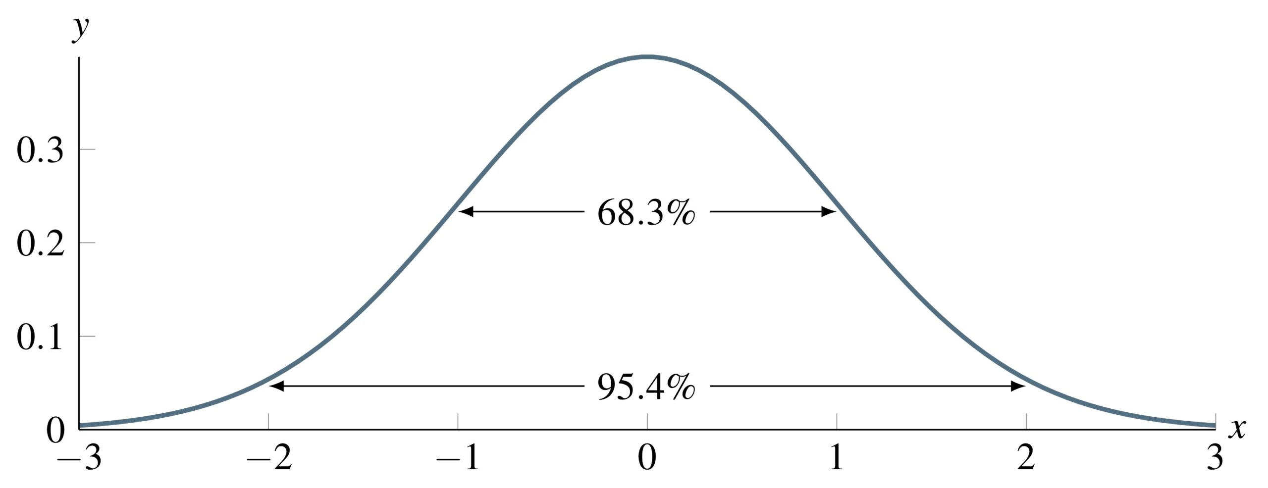
In practice, the probability of generating a given noise value should be weighted so that values closer to 0 are more likely than values at the tails. One way of achieving this is with a standard normal density function, a “bell-shaped” curve that will be familiar to anyone who has taken a statistics course (see figure below). The probability of generating a number between numbers a and b is equal to the area under the function between the x values of a and b; that is, the integral of the standard normal density function. Because the density function is taller near zero, the probability of generating a number near zero is higher, and this probability decreases the farther we move from zero. There is approximately a 68.3% probability of generating a number between -1 and 1, and a 95.4% probability of generating a number between -2 and 2.

We can therefore obtain a random noise value in the range from -marginOfError to marginOfError with approximately 95% probability by generating a pseudorandom decimal according to the standard normal density function, and then multiplying this number by marginOfError/2. But how can we produce these numbers?

Remember our classic text for computing random numbers in the pre-computing era, A Million Random Digits with 100,000 Normal Deviates? The book earns the second half of its name because it contains 100,000 random numbers sampled underneath the standard normal density function. Fortunately, we won’t need to consult a 70 year-old book because programming languages will include a function RandNormal() that returns a random number according to the standard normal density function, allowing us to update our implementation of AddNoise() as follows.

AddNoise(poll, marginOfError)
    x ← RandNormal()
    x ← x/2 (95% chance of x being between -1 and 1)
    x ← x * marginOfError (now x is in range)
    return x + poll

And just like that, we are done! Note how we saved the hardest part of our work, incorporating randomness into polling data, until last? We will say more on this principle in the next chapter.

It’s time to code

For now, it is time to implement our work in this chapter and simulate an election from polling data. We will then return to analyze the results of this simulation and reflect on the nature of simulation in this chapter’s conclusion.