Setup
In what follows, “write and implement” means that we suggest that you write the function in pseudocode first, and then implement your function.
To get started, create a folder named practice1 under your src coding directory. Then, place your code for this assignment within this folder.
Check your work with our autograders
If you are logged in to our course on Cogniterra, then you can find the practice problems for this chapter linked in the window below, where you can enter your code into our autograders and get real time feedback. You can also view these exercises using a direct link. Beneath this window, we provide a full description of all this chapter’s exercises.
Metagenomics Functions Part 1: Alpha Diversity
It may come as a surprise, but over half of the cells in your body are bacteria! And a recent estimate pegged the number of microbial species on Earth at 1 trillion. It is starting to become apparent that this is a microbial planet that we just happen to inhabit.
The community of microbes present in some habitat is called that community’s microbiome. Many current studies are examining the microbiome of all sorts of locations, from deep sea vents to the International Space Station, and from the New York City subways to the human body, in an effort to determine the unseen diversity present everywhere on our planet.
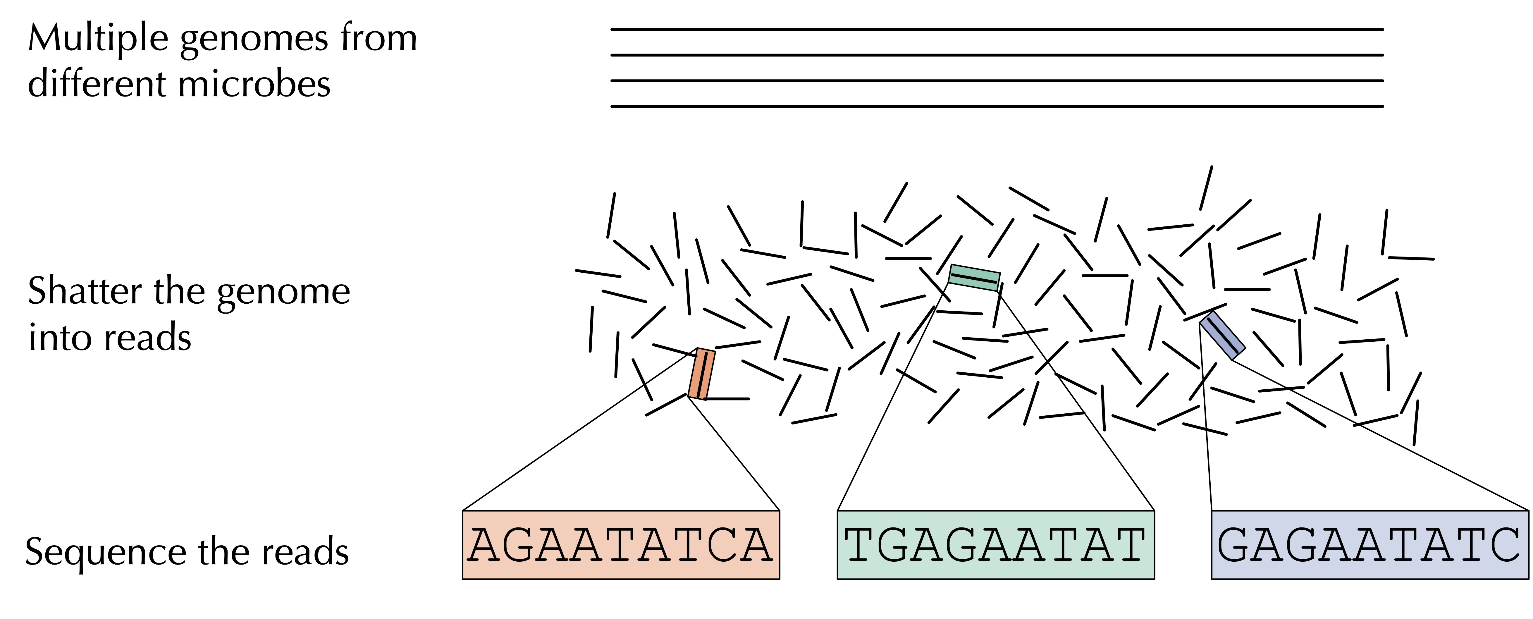
Microbiome studies have been enabled by the era of affordable DNA sequencing and have given rise to the field of metagenomics, which is the study of DNA (or RNA) recovered from some environmental sample. As illustrated in the figure below, once we isolate DNA captured from this environment of interest, which may derive from hundreds or thousands of different organisms, we shatter that DNA into fragments, which we feed into a sequencing machine that is capable of reading these short DNA fragments, called reads.
For a given sample, we are left with something of a “DNA stew”, or a conglomeration of DNA strings whose species identity is unknown.
STOP: How should we store the collection of strings for a single metagenomics sample?
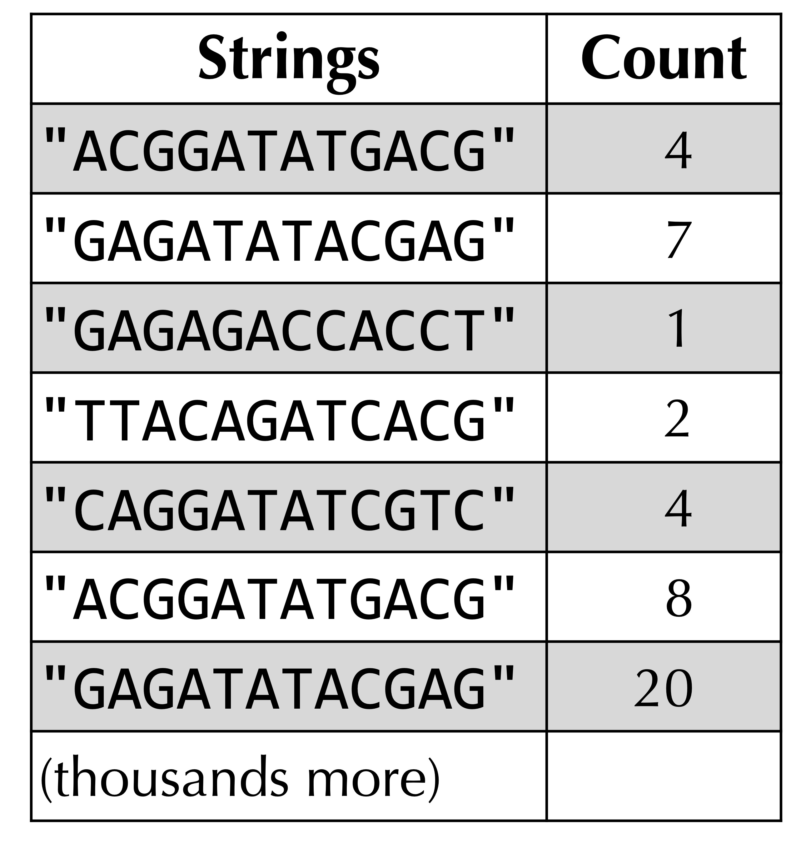
One way to store the DNA stew corresponding to a single metagenomics sample is to use an array of strings, but because the sample may have duplicated strings, we will use a data structure that we have already worked with in this chapter: the frequency table!
For example, the figure below shows the frequency table for a hypothetical collection of DNA strings. (In practice, each DNA string will have hundreds or thousands of nucleotides.)
Now that we know how we plan to represent a metagenomics sample using a frequency table, we would like to analyze that sample. One natural scientific question we can ask is how diverse the sample is, which is called the alpha diversity. The issue presented to us is how we can quantify this hazily defined notion of a sample’s diversity.
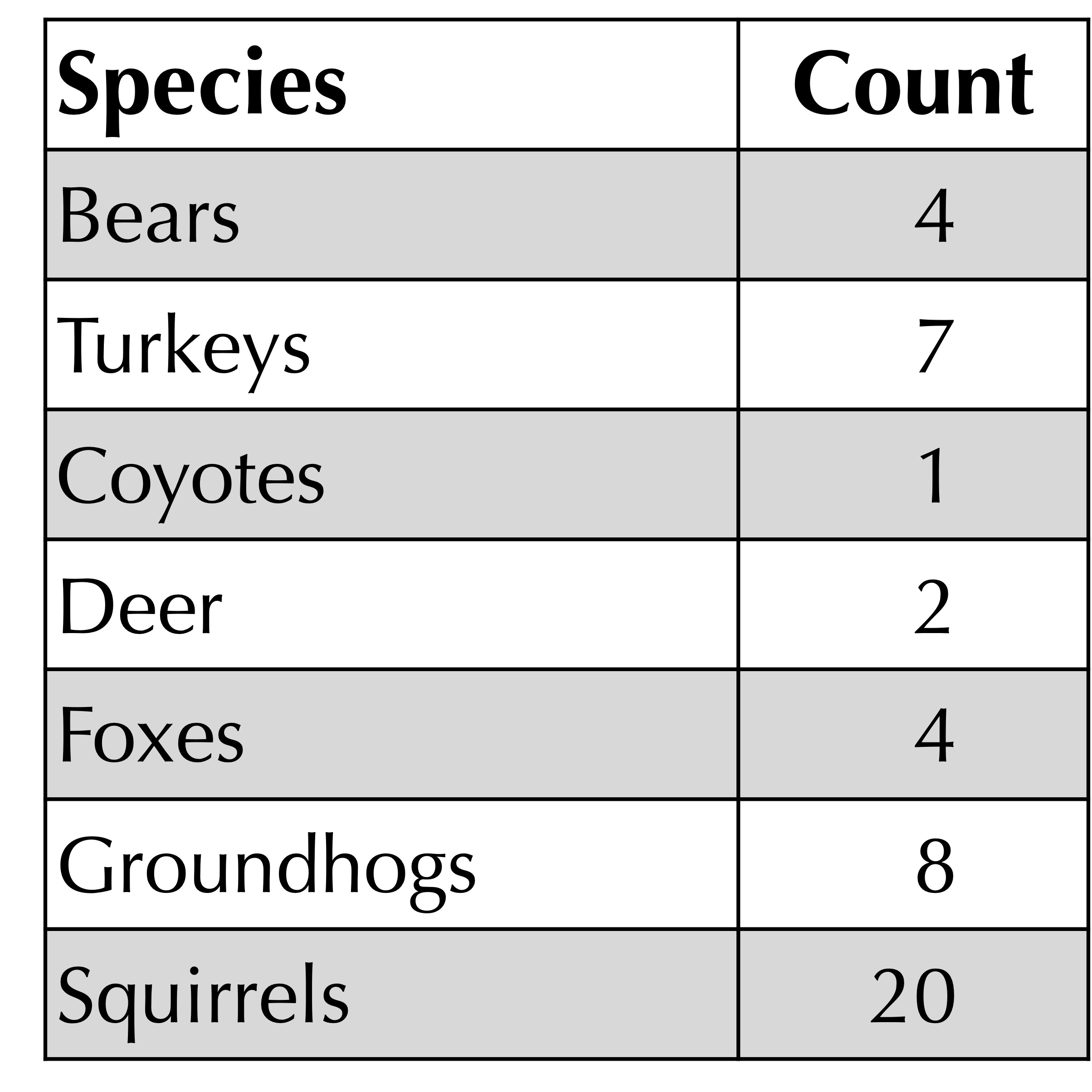
Quantifying alpha diversity is an old question that vastly predates the era of metagenomics. Biologists have long studied ecosystems by counting the number of organisms from each species in a given location. For example, the figure below shows a hypothetical catalog of organisms present in a habitat in western Pennsylvania. It’s just a frequency table!
One metric of a habitat’s alpha diversity is richness, which is a fancy term for the number of species present in the habitat (i.e., the number of elements in the frequency table with positive counts). For example, the richness of the habitat below has been measured to be equal to 7.
We are now ready to write a function that determines the richness of a given frequency table.
Code Challenge: Implement a function.Richness()
Input: a frequency tablemapping strings to their number of occurrences.sample
Return: the richness of.sample
Richness is not a great measure of alpha diversity for a few reasons. For one, just because a species or string was not detected in a sample does not mean that it does not exist in the habitat.
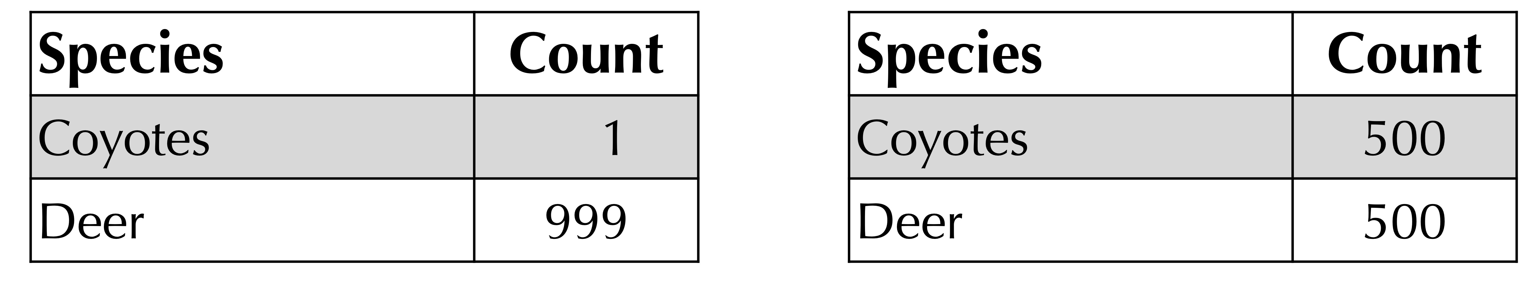
Furthermore, consider the following extreme example of frequency tables for two different habitats. They both have richness equal to 2 but are clearly very different because the habitat on the right is more even than the one on the left and therefore has greater alpha diversity.
To move toward a quantification of alpha diversity, consider the jar below containing six balls of three different colors. Say that we draw a ball from this jar, replace it, and then draw another ball (all without looking). What is the probability that we drew a green ball twice?
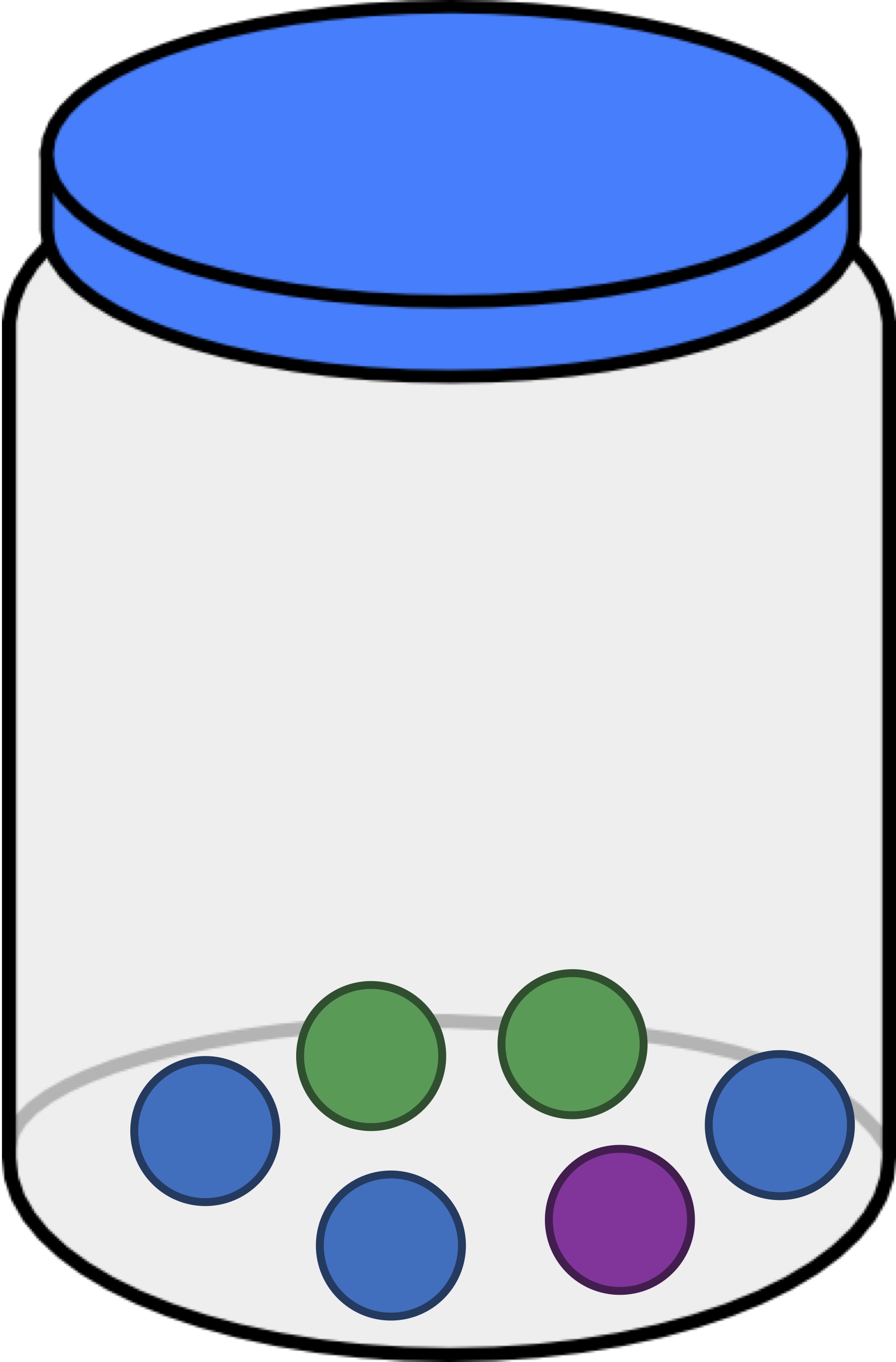
Since the jar contains two green balls, the likelihood of the first ball being green is 2/6. And because we replaced the ball, the same is true for the likelihood of the second ball being green. As a result, the probability that we draw a green ball twice is equal to (2/6) · (2/6) = (4/36) = (1/9).
Exercise: If we draw a ball from the jar, replace it, and draw a ball again, what is the probability of drawing a purple ball twice? Express your answer as a decimal to four decimal places.
Next, say that we draw a ball from the jar, replace it, and draw another ball. What is the probability that both balls that we drew have the same color, regardless of what that color is?
This probability is equal to the sum of three probabilities: the probability that both drawn balls are green, the probability that both drawn balls are purple, and the probability that both drawn balls are blue. These probabilities are equal to (1/9), (1/36), and (1/4), respectively, and so our desired probability is 1/4 + 1/9 + 1/36 = 7/18 = 0.3888…
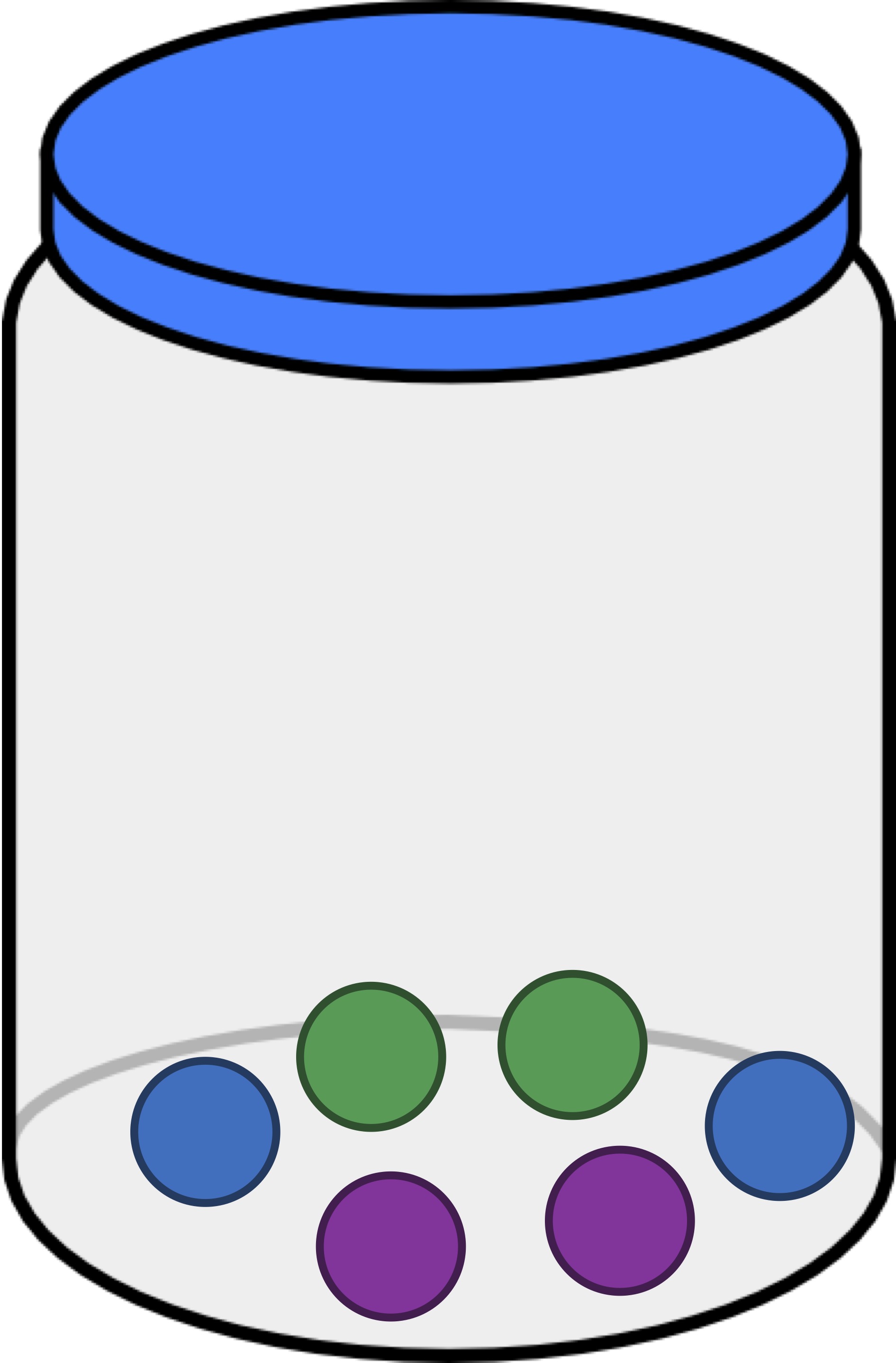
Next, we will alter the jar so that it contains two balls of each color (see figure below). This time, for each individual color, the likelihood of drawing two balls of this color is equal to 1/9. Because there are three colors, the probability of drawing two balls of the same color (assuming that we replace the first ball) is equal to 1/9 + 1/9 + 1/9 = 1/3.
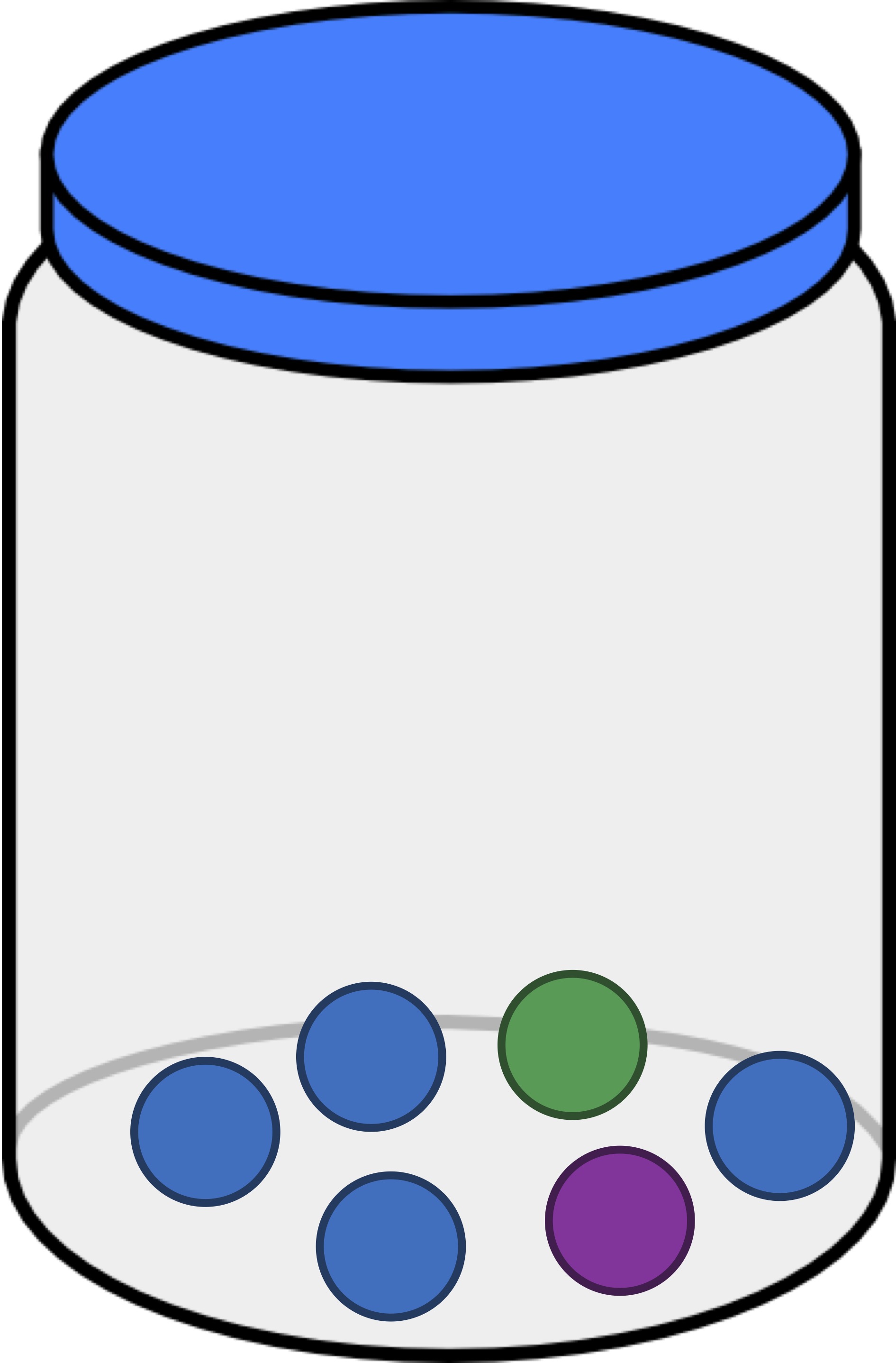
Exercise: The jar in the figure below contains one green ball, one purple ball, and four blue balls. If we draw a ball, replace it, and draw a ball again, what is the probability that the two drawn balls have the same color? Express your answer as a decimal.
We can think of each of the three jars that we have introduced (reproduced below) as a habitat containing differing numbers of objects. As a result, we ask ourselves, which of these three jars is the most even? Intuitively, this should be the jar that contains three balls of each color, shown below in the middle. The jar that is the least even is the one on the right, since it is dominated by blue balls.
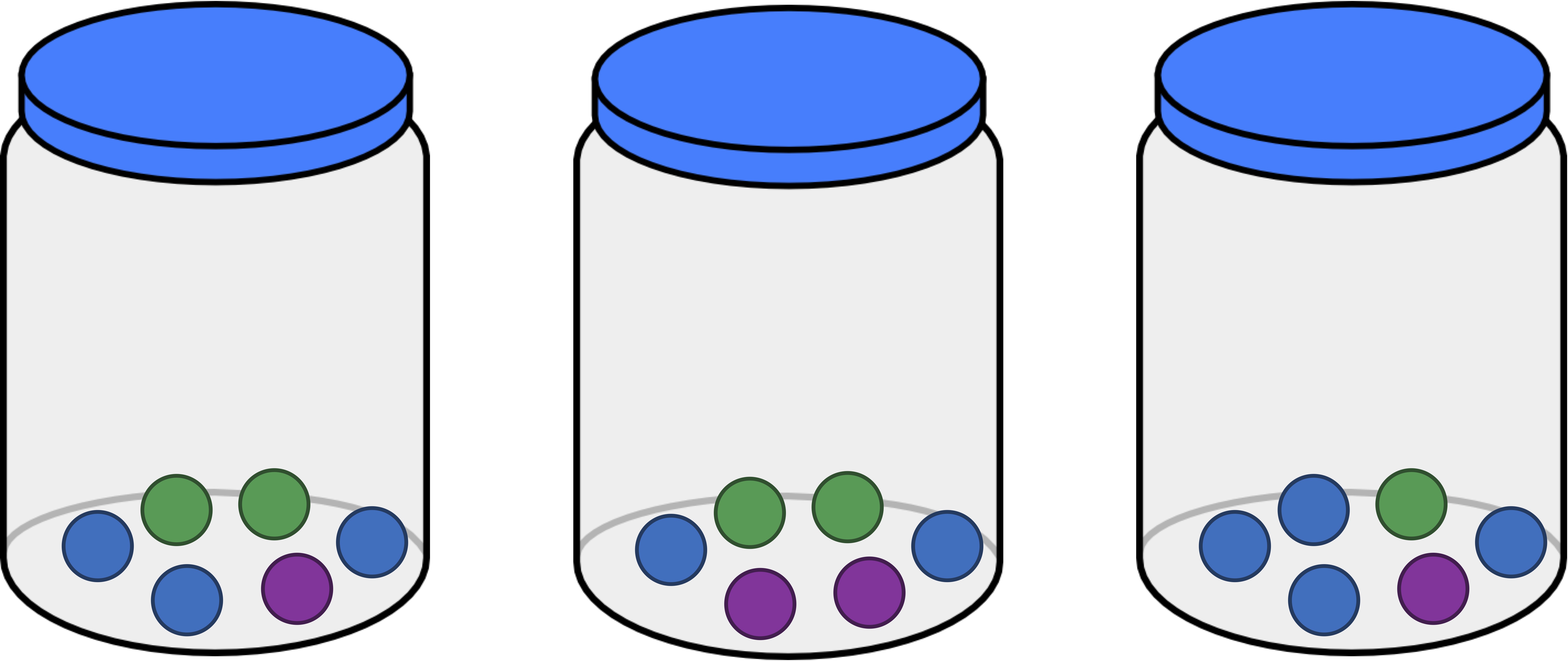
Evenness is connected to our discussion of drawing balls from jars because the less even a sample, the more likely it is that we would “draw the same type of object twice” from this sample. As a result, the probability of drawing the same type of object twice (assuming the first object is replaced) gives us a metric that has an inverse relationship with evenness: the larger this probability, the less even the sample.
In general, the probability of choosing two objects (with replacement of the first object) from a sample of the same type is called Simpson’s index in honor of Edward Simpson, who introduced this metric in 1949.
To demonstrate the utility of Simpson’s index, consider the two hypothetical coyote-deer habitats that we introduced earlier, reproduced below. Although these two habitats have the same richness, their Simpson’s index is very different; the Simpson’s index of the habitat on the left is equal to (1/1000)2 + (999/1000)2 = 0.998, and the Simpson’s index of the habitat on the right is equal to (1/2)2 + (1/2)2 = 0.5.
STOP: What is the smallest or largest that Simpson’s index could ever be for an ecosystem?
The least even possible frequency table is one having richness equal to 1. In this case, we will always draw two objects having the same instance, and so the maximum possible value of Simpson’s index is equal to 1.
On the other side of the spectrum, the most even possible frequency table with n elements is one that has equal numbers of each “species”. For such a frequency table, the likelihood of selecting a member of a given species twice is (1/n)2, so that the Simpson’s index is equal to n · (1/n)2 = 1/n. As the number of species (n) in such a sample increases, the lowest possible Simpson’s index of a sample heads toward zero.
Before implementing a function to compute the Simpson’s index, we pause to provide an exercise that we suggest will be helpful as a subroutine when implementing a Simpson’s index function.
Code Challenge: Implement a function.SumOfValues()
Input: a frequency tablemapping strings to integers.sample
Return: the sum of all values in.sample
Code Challenge: Implement a function.SimpsonsIndex()
Input: a frequency tablemapping strings to integers.sample
Return: the Simpson’s index of.sample
Metagenomics Functions Part 2: Beta Diversity
Now that we have seen two methods of quantifying the alpha diversity of a single sample, we turn our attention to determining how different two samples/habitats are. This diversity between samples is called the beta diversity between the samples; as with alpha diversity, we will attempt to quantify this measure.
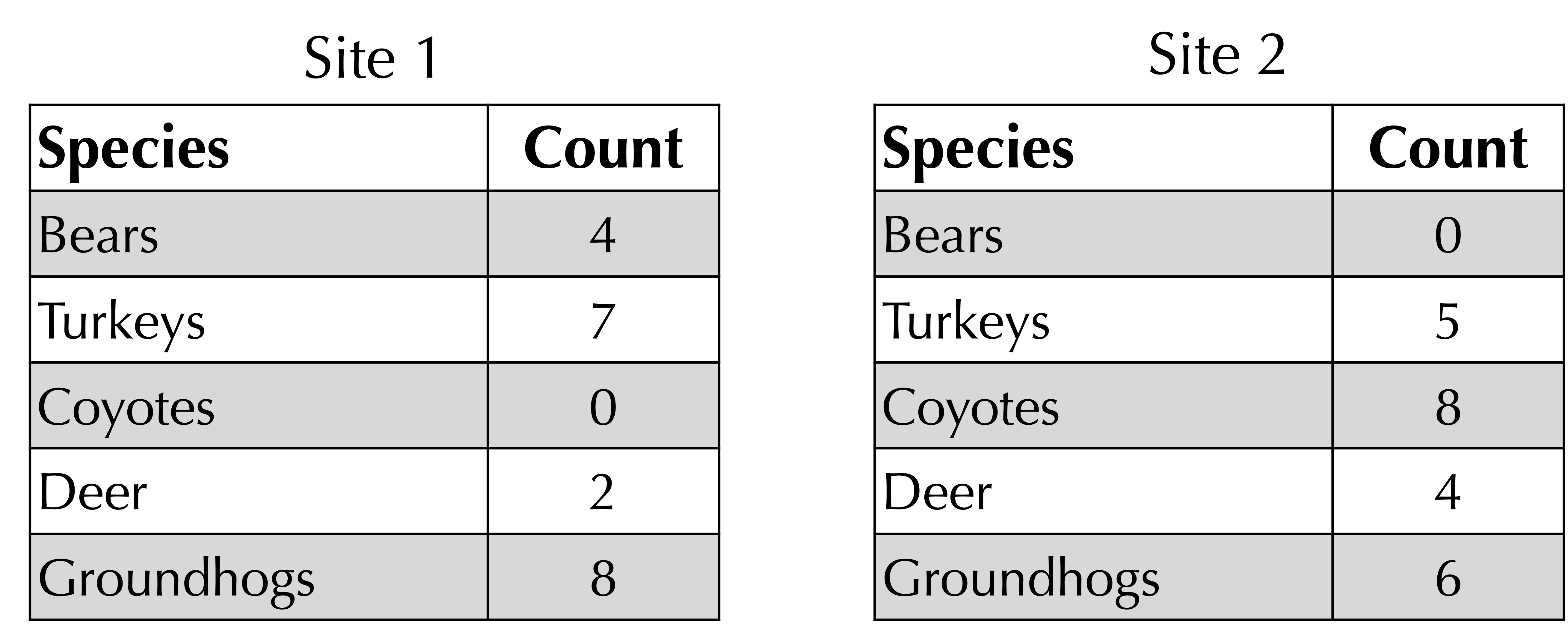
STOP: Consider the following two frequency tables for hypothetical habitats in western Pennsylvania. How could we quantify the beta diversity of these habitats?
As was the case with alpha diversity, measuring beta diversity is an old biological question that predates the genome sequencing era.
One idea for quantifying the beta diversity between two sites would be to take the difference between the Simpson’s index of the two sites. The greater this difference, perhaps the greater the difference between the two sites.
Yet consider two habitats, one with 999 coyotes and 1 deer, and the other with 1 deer and 999 coyotes. We know that both of these habitats have Simpson’s index equal to 0.998, and yet they are clearly very different. (For a more extreme example, one habitat could have 1 deer and 999 coyotes, and the other habitat could have 1 gorilla and 999 aliens.)
Another way of measuring the beta diversity between two sites would take the ratio of the number of species that are present only at one site to the total number of species across two sites. For example, consider the two sites presented previously. Two species (coyotes and bears) are present only at one site, as shown by the elements in the frequency tables having zero counts. There are five total species across both sites. Therefore, the ratio between non-shared species and total species is 2/5.
STOP: This approach is a flawed way of differentiating two ecosystems. Why?
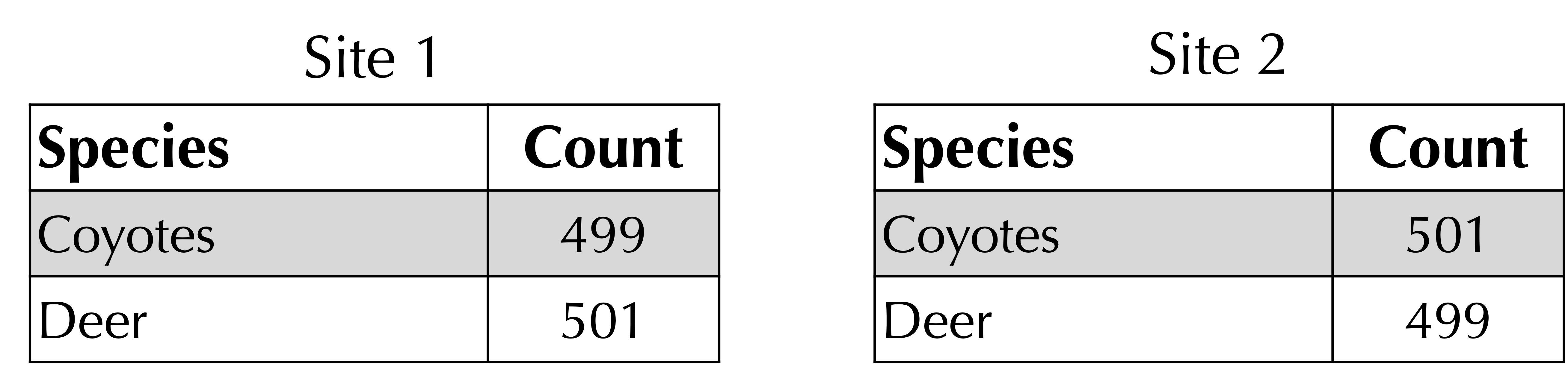
Consider once again our two hypothetical coyote-deer ecosystems, one with 1 coyote and 999 deer, and the other with 500 of each animal. These habitats have two total species, neither of which is present only in one; as a result, these two habitats would have a beta diversity “distance” value equal to zero! And yet these two habitats are very different …
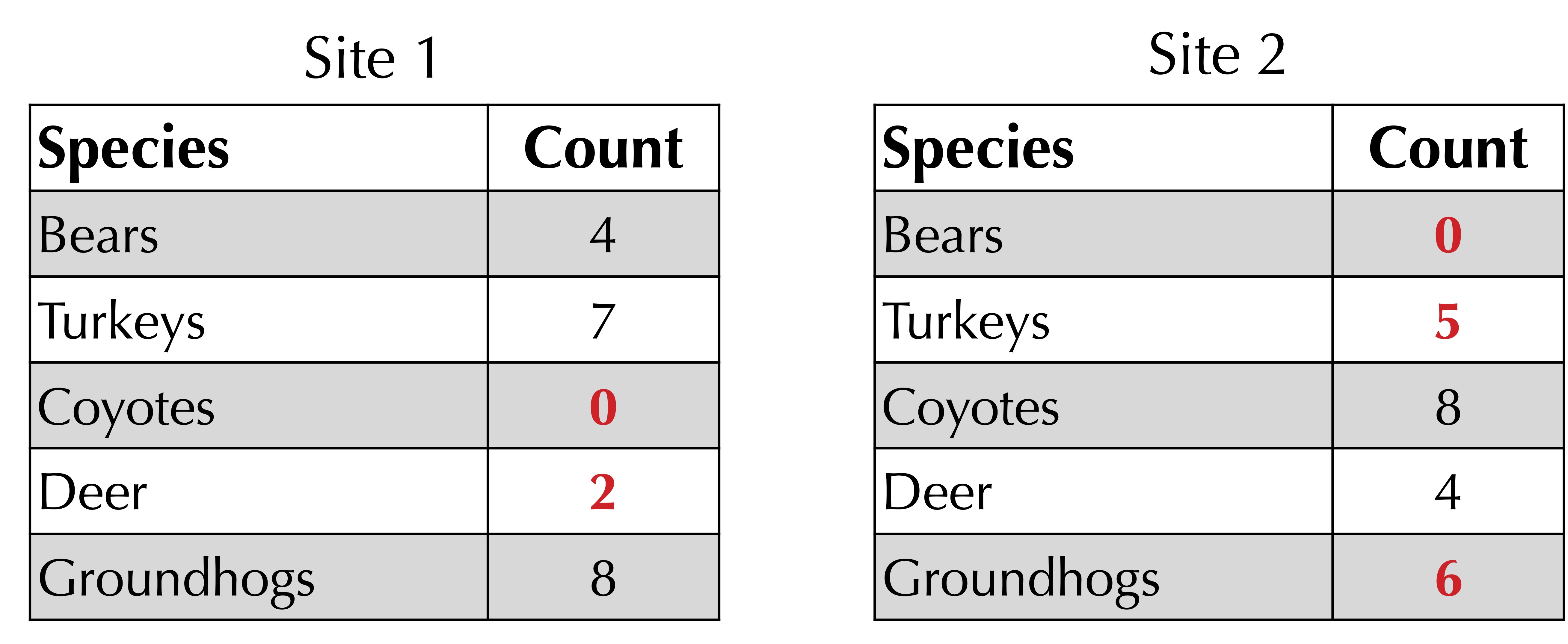
To obtain a better metric for beta diversity, we turn to a function developed by J. Roger Bray and John Curtis in 1959 when studying the Wisconsin forest. Given two frequency tables, sum the minimum count of each species in each row. For our ongoing example, illustrated in the figure below, this sum of corresponding minimum values is equal to 0 + 5 + 0 + 2 + 6 = 13. (Note: if a species is not present in a frequency table, we can assume that its count is equal to zero.)
Next, take the average of the total counts at each site. As shown in the figure below, this total is 21 for site 1 and 23 for site 2, yielding an average of (21 + 23)/2 = 22.
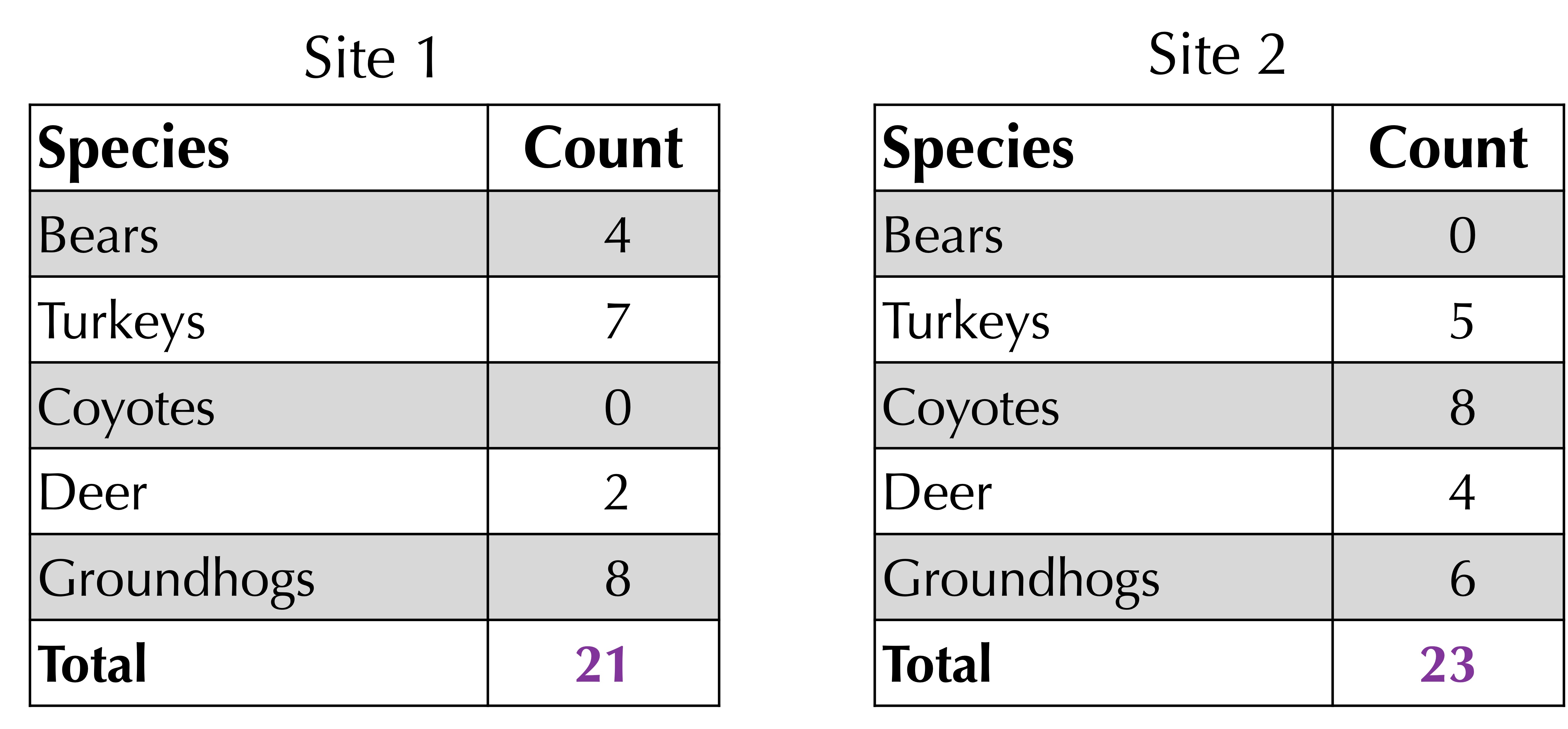
The Bray-Curtis distance is 1 minus the sum of corresponding minimum values divided by the average of the total values. For the above example, the Bray-Curtis distance is 1 – 13/22 = 9/22.
Although the Bray-Curtis distance is an excellent metric of beta diversity, it is not the only one. One such alternative is called the (weighted) Jaccard distance and is defined as follows.
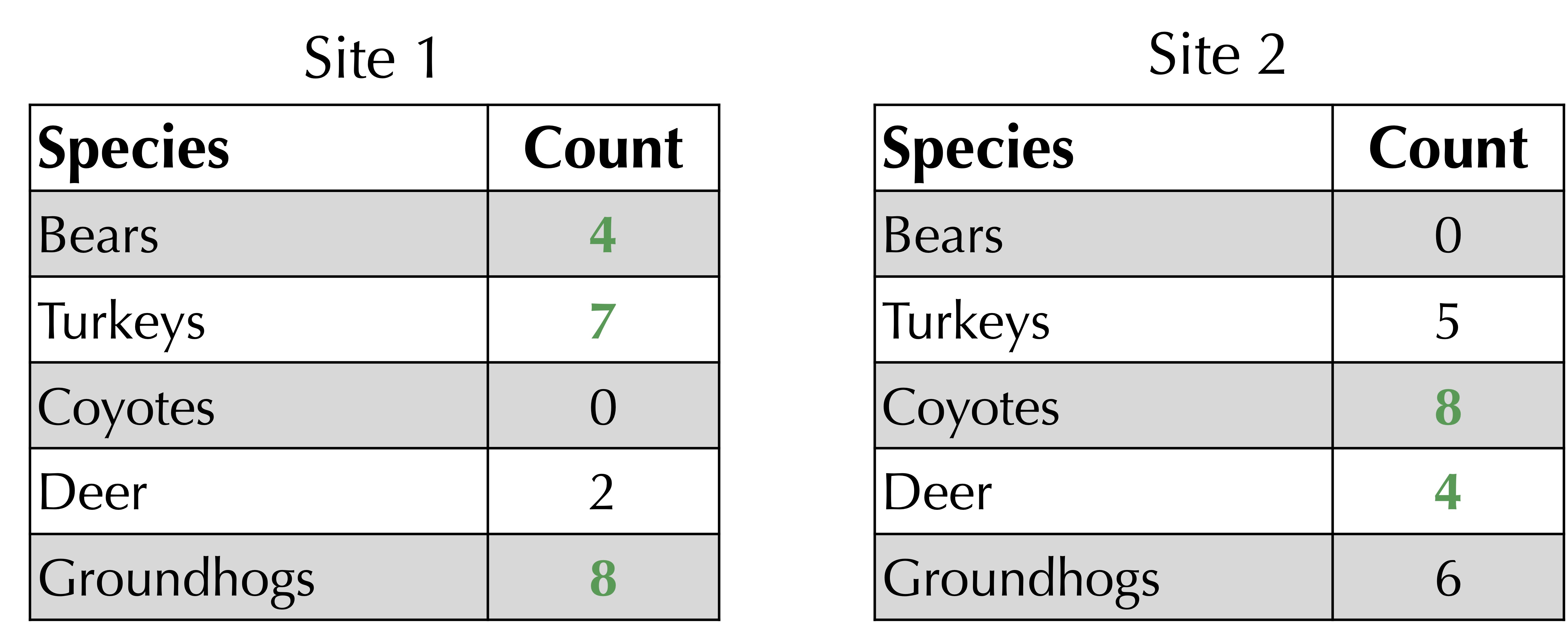
First, sum the maximum of the two values in corresponding rows of the frequency tables. As shown below, for our ongoing example, this sum of maxima is equal to 4 + 7 + 8 + 4 + 8 = 31.
The Jaccard distance is 1 minus the sum of corresponding minimum values (computed above) divided by the sum of corresponding maximum values. For the ongoing example, the Jaccard distance is equal to 1 – 13/31 = 18/31.
As with alpha diversity, both the Bray-Curtis and Jaccard distances have possible values ranging from 0 to 1. The closer the distance is to 0, the more similar the habitats. The closer the distance is to 1, the more different the habitats.
For example, consider the following two sites, which are very similar. Their Bray-Curtis distance is 1 – (499 + 499)/1000 = 2/1000, and their Jaccard distance is 1 – (499 + 499)/(501 + 501) = 4/1002.
Although habitats with similar numbers of species will have a small value of both the Bray-Curtis and Jaccard distances, we should also ensure that habitats that are different have large distance values for both functions.
Exercise: Consider one site with 1 coyote and 999 deer, and another site with 500 of each animal. Compute the Bray-Curtis and Jaccard distances between these sites. Are they similar?
Before implementing the Bray-Curtis and Jaccard distance functions, we pause to make one more point. Consider the two habitats in the figure below. Are they similar or different?
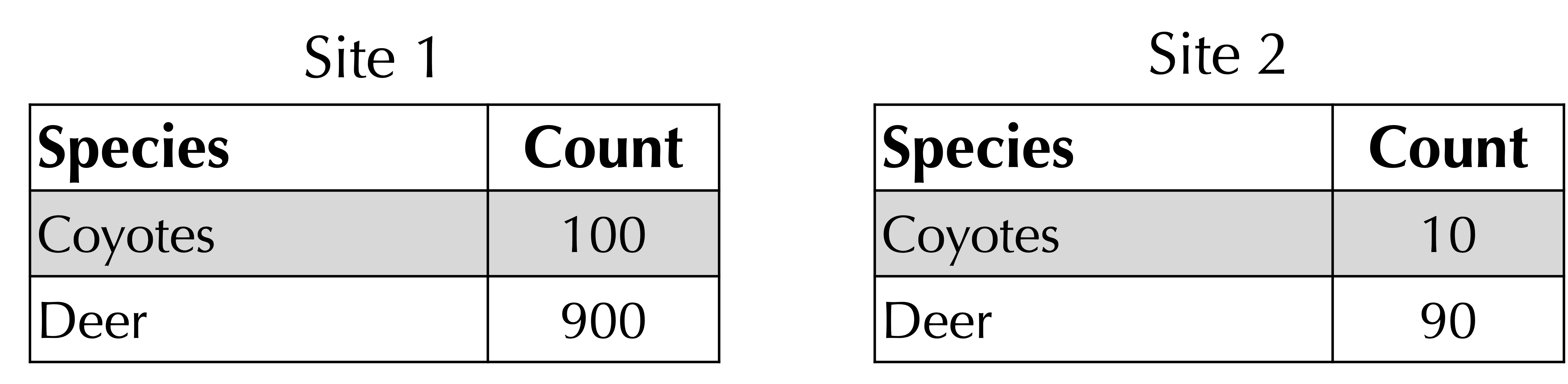
If we consult the Bray-Curtis and Jaccard distances, we find that these distances are respectively 450/550 and 900/1000. And yet the ratio of coyotes to deer at each site is the same!
If we want to account for the absolute numbers at each site, then the Bray-Curtis and Jaccard distances are suitable. If we want to account for the relative numbers at each site, then we should consider normalizing the samples by dividing every element in one frequency table by a number so that the values in each table has the same sum. In this case, we could divide the counts in site 1 by 10.
Real metagenomics experiments often use a different approach called undersampling, if we collect n DNA strings from site 1 and m DNA strings from site 2 with n > m, then we randomly choose m strings from site 1 and discard the rest.
We are now nearly ready to implement the Bray-Curtis and Jaccard distances. First, we provide the Bray-Curtis distance as a function in pseudocode below. Note that this function calls the function SumOfValues()SumOfMinima()
BrayCurtisDistance(sample1, sample2)
    total1 ← SumOfValues(sample1)
    total2 ← SumOfValues(sample2)
    average ← (total1 + total2)/2
    sum ← SumOfMinima(sample1, sample2)
    return 1 - sum/average
Code Challenge: Implement.SumOfMinima()
Input: two frequency tablesandsample1mapping strings to their number of occurrences.sample2
Return: the sum of corresponding minimum values ofandsample1.sample2
Code Challenge: Implement.BrayCurtisDistance()
Input: two frequency tablesandsample1mapping strings to their number of occurrences.sample2
Return: The Bray-Curtis distance betweenandsample1.sample2
Next, we focus on the Jaccard distance. This function also uses the SumOfMinima()SumOfMaxima()
JaccardDistance(sample1, sample2)
    sumMin ← SumOfMinima(sample1, sample2)
    sumMax ← SumOfMaxima(sample1, sample2)
    return 1 - sumMin/sumMax
Code Challenge: Implement.SumOfMaxima()
Input: two frequency tablesandsample1mapping strings to their number of occurrences.sample2
Return: the sum of corresponding maximum values ofandsample1.sample2
Code Challenge: Implement.JaccardDistance()
Input: two frequency tablesandsample1mapping strings to their number of occurrences.sample2
Return: The Jaccard distance betweenandsample1.sample2
Up Next
It may surprise you that you now have most of the basics of programming under your belt. Regardless of how sophisticated a program is, or how many lines of code it has, it is built upon these fundamentals.
In the next chapter, we will learn about a modeling paradigm called “Monte Carlo simulation” in which we incorporate randomized simulations to make a prediction. Specifically, we will turn our attention to how we can use Monte Carlo simulation to forecast a presidential election.