Some Gritty Details about DNA Replication

Lurking biological phenomenon or statistical fluke?

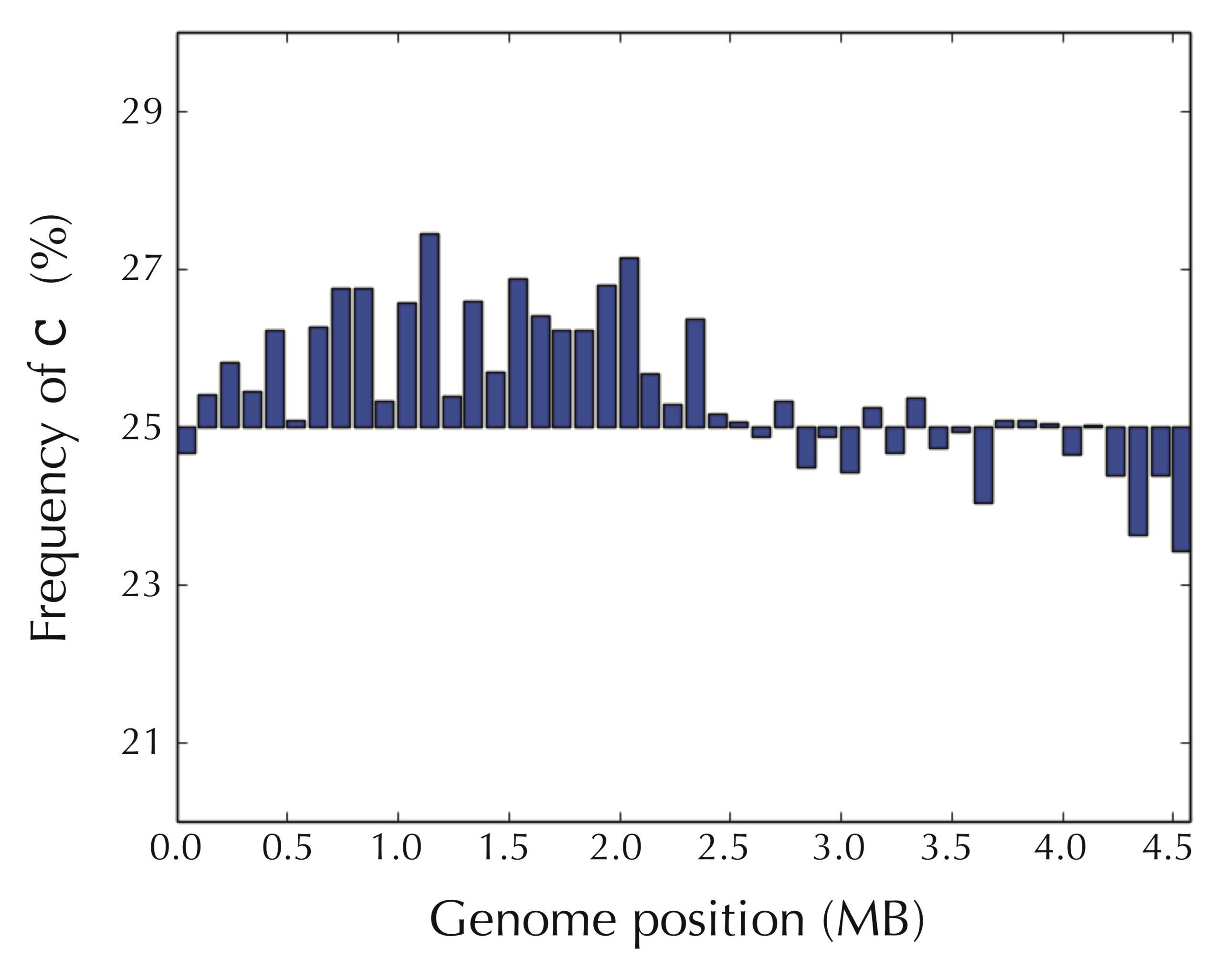
The figure below reveals a surprising pattern. We have partitioned the E. coli genome into 46 equally sized windows of approximately 100,000 nucleotides, starting at the experimentally verified terminus of replication, and then computed the frequency of cytosine in each window. For the first half of the genome, most windows have a high cytosine frequency (significantly above 25%), whereas most windows after we reach ori have a lower cytosine frequency (significantly below 25%).

The frequency of cytosine in 46 equally sized windows of approximately 100,000 nucleotides each in the *E. coli* genome. The first half of the windows tend to have high cytosine frequency, and the second half tend to have low cytosine frequency.

In contrast, as shown in the figure below, the picture is reversed for guanine frequency. After we pass ori, most windows have high guanine frequency.

The frequency of guanine in the same 46 windows in the *E. coli* genome. Half of the genome has windows that tend to have low guanine frequency, and half of the genome has windows with high frequency. However, the picture is reversed from the preceding figure and the consideration of cytosine.

We obtain an even more striking visualization if we take the difference of the frequencies of guanine and cytosine in each window, as shown in the figure below.

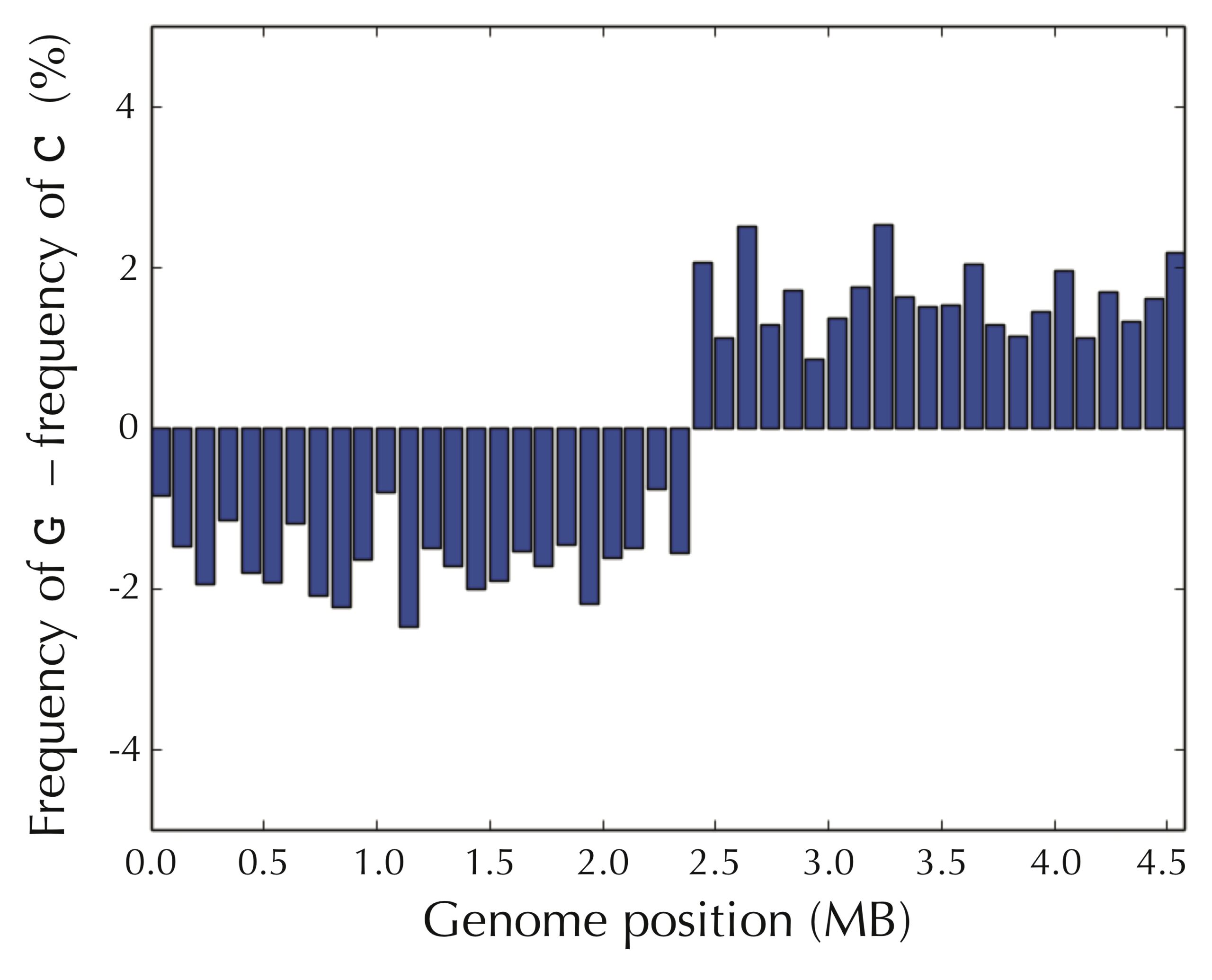
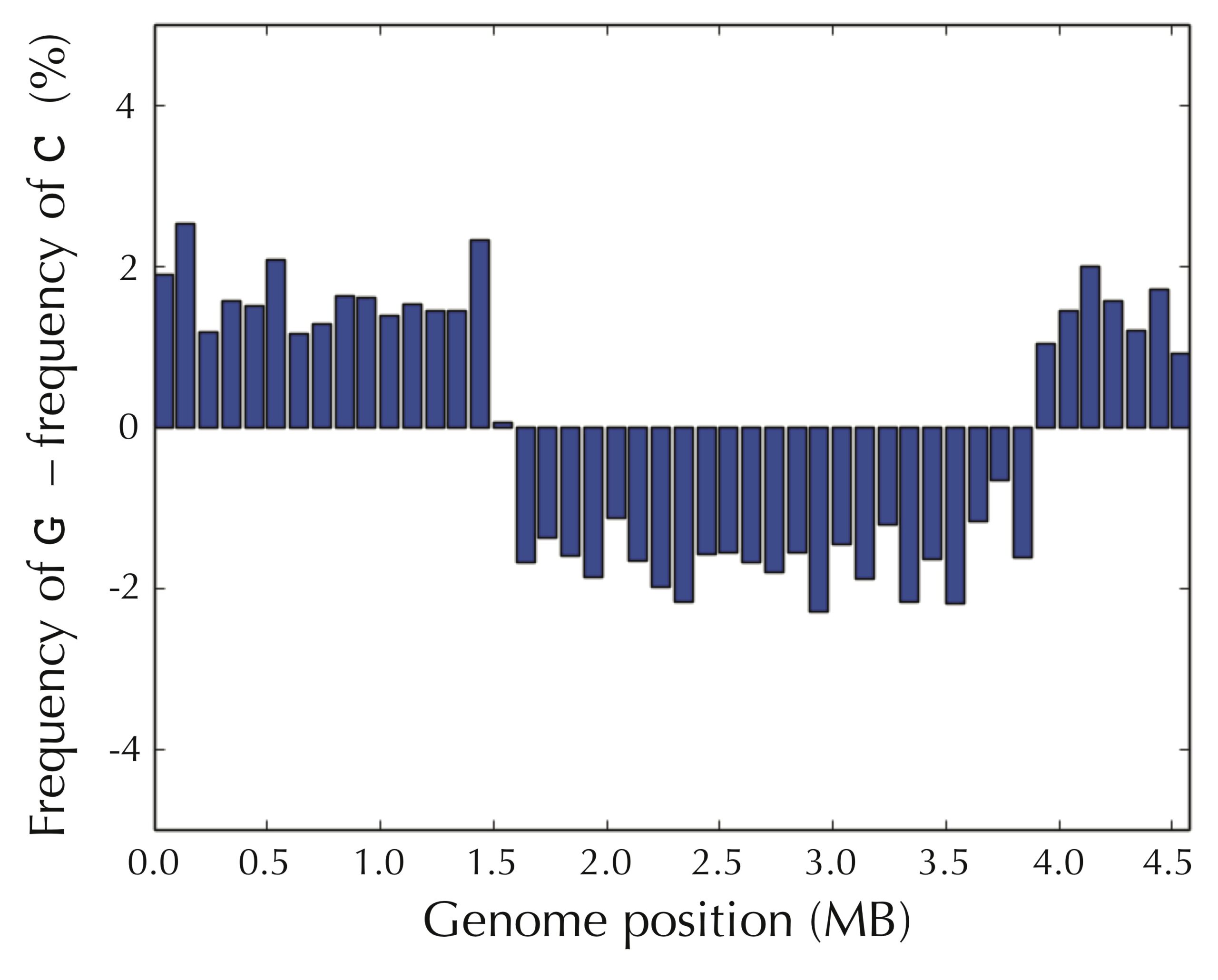
The difference between the frequencies of guanine and cytosine across the 46 windows of the *E. coli* genome, assuming that the genome begins at the experimentally verified replication terminus of *E. coli*.

Even if we assume that we do not know the location of ori in advance, the pattern still presents itself when starting at an arbitrary position of the E. coli genome, as shown in the figure below.

The difference between the frequencies of guanine and cytosine across the 46 windows of the *E. coli* genome, starting at an arbitrary position of the genome.

It seems that we have uncovered a hint about how to find ori — we can simply walk along the genome and check where the difference between the frequency of guanine and cytosine switches from negative to positive! But why in the world would such a simple test allow us to find the replication origin of a bacterium?

The simplest way to replicate a genome

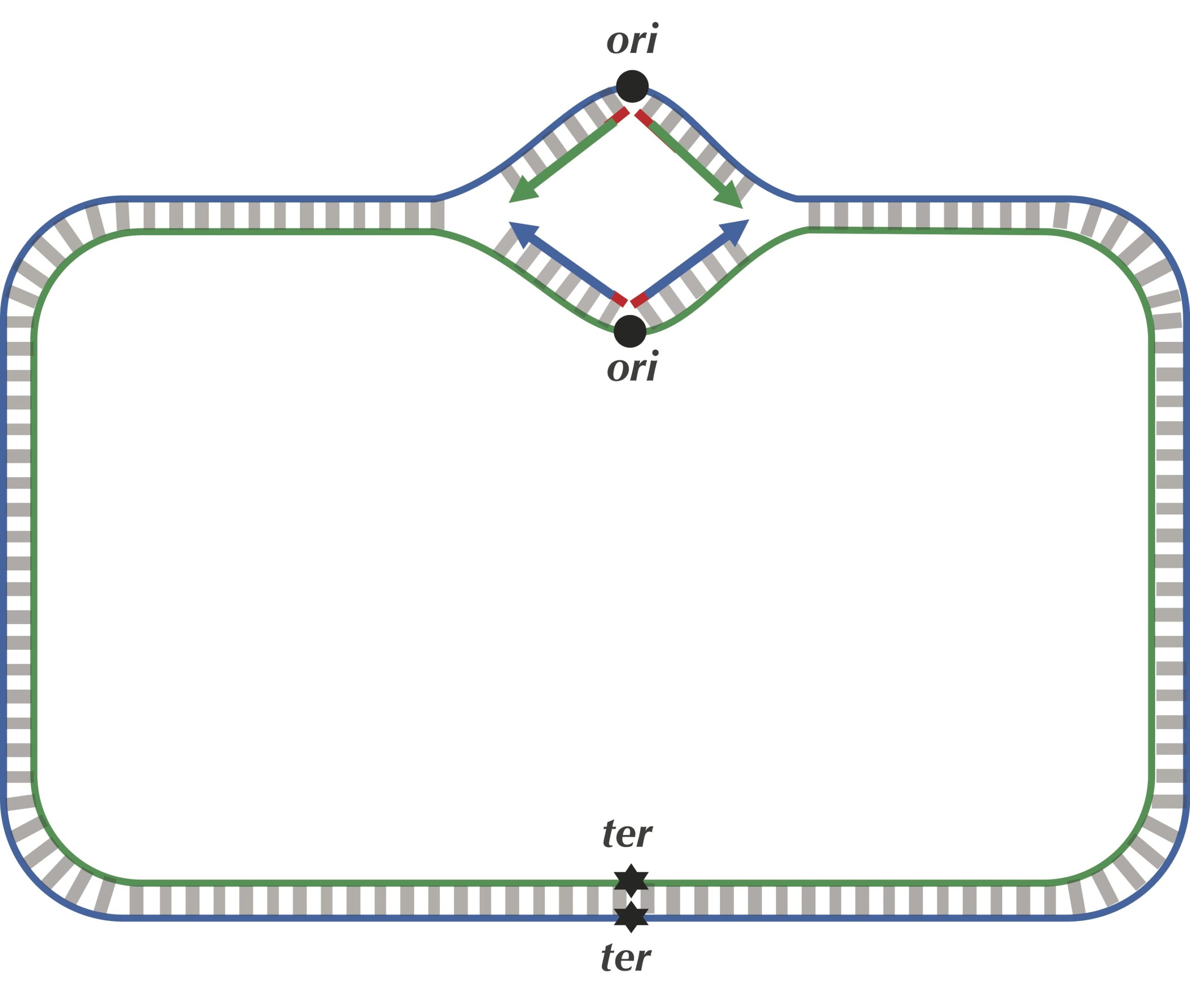
We are now ready to discuss the replication process in more detail. As illustrated in the figure below, the two complementary DNA strands running in opposite directions around a circular chromosome unravel, starting at ori. As the strands unwind, they create two replication forks, which expand in both directions around the chromosome until the strands completely separate at the replication terminus (denoted ter). The replication terminus is located roughly opposite to ori in the chromosome.

Four imaginary DNA polymerases at work replicating a chromosome as the replication forks extend from *ori* to *ter*. The blue strand is directed clockwise, and the green strand is directed counterclockwise.

The problem with our current description is that it assumes that DNA polymerases can copy DNA in either direction along a strand of DNA (i.e., both 5′ → 3′ and 3′ → 5′). However, nature has not yet equipped DNA polymerases with this ability, as they are unidirectional, meaning that they can only traverse a template strand of DNA in the 3′ → 5′ direction. Notice that this is opposite from the 5′ → 3′ direction in which DNA is read.

STOP: If you were a unidirectional DNA polymerase, how would you replicate DNA? How many DNA polymerases would be needed to complete this task?

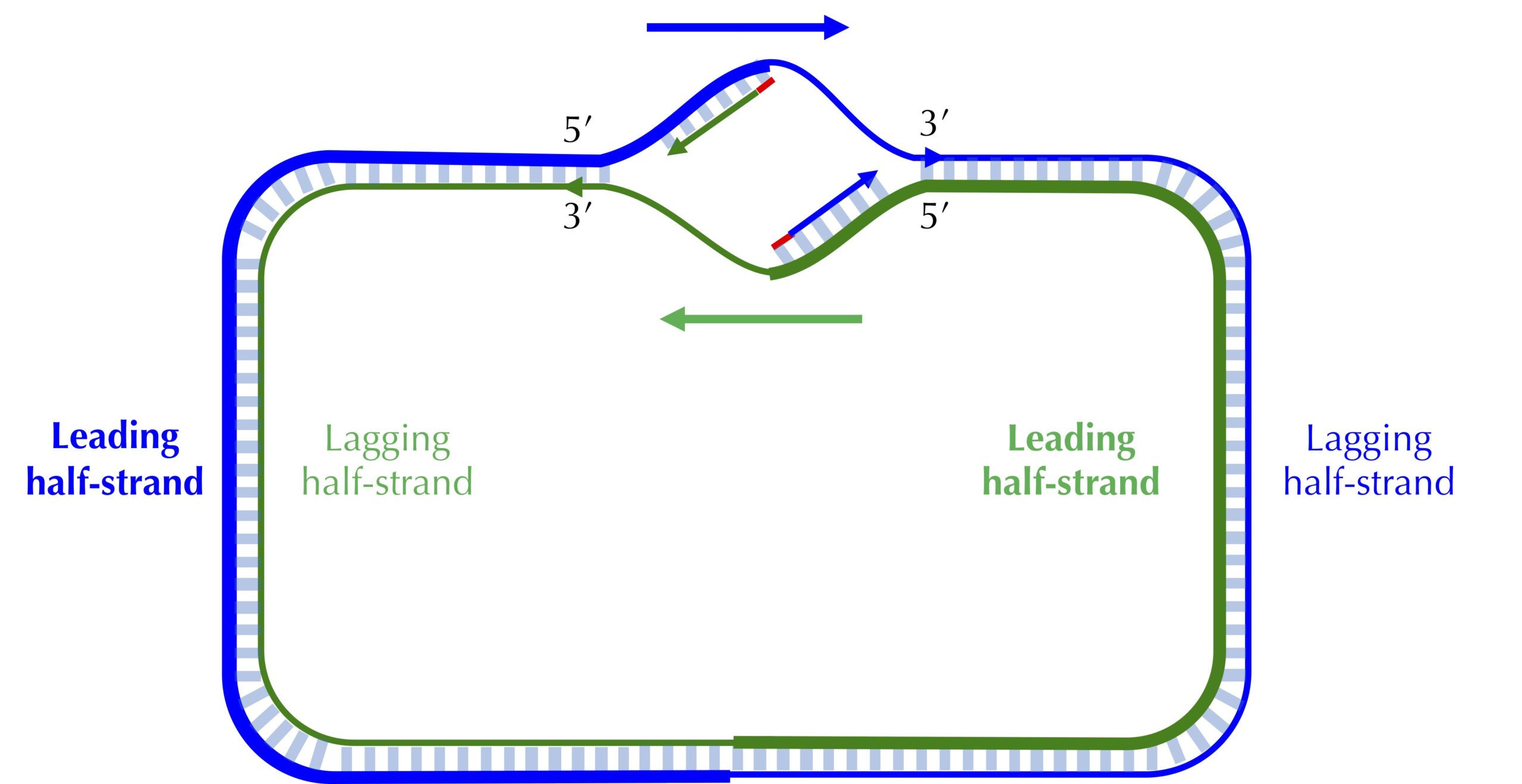
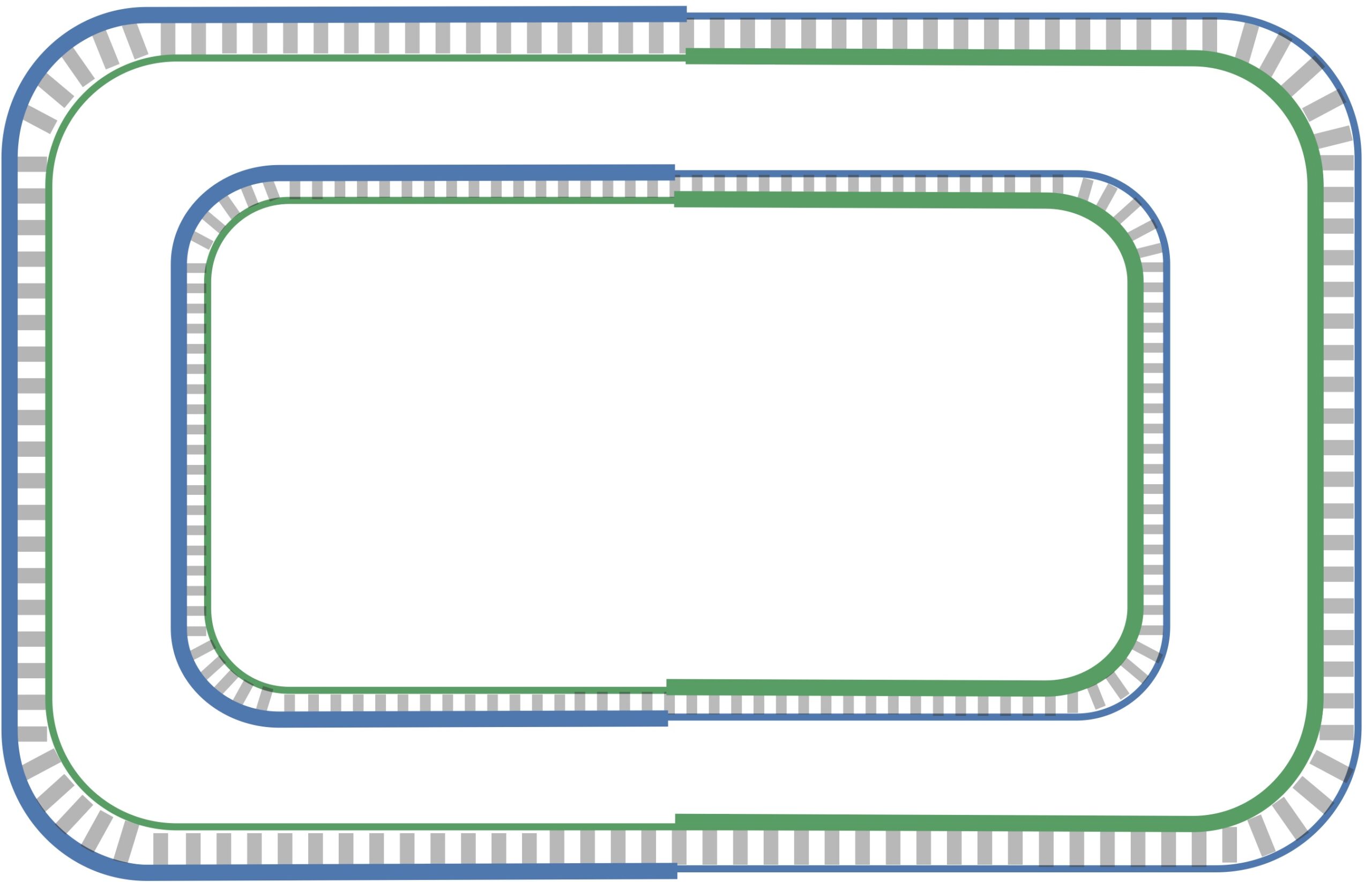
The unidirectionality of DNA polymerase requires a major revision to our naive model of replication. Imagine that you decided to walk along DNA from ori to ter. There are four different half-strands of parent DNA connecting ori to ter, as highlighted in the figure below. Two of these half-strands are traversed from ori to ter in the 5′ → 3′ direction and are called lagging half-strands (represented by thin blue and green lines in the figure below). The other two half-strands are traversed from ori to ter in the 3′ → 5′ direction and are called leading half-strands (represented by thick blue and green lines in the figure below).

Complementary DNA strands with lagging and leading half-strands shown as thin and thick lines, respectively.

Asymmetry of replication

While biologists will feel at home with the following description of DNA replication, computer scientists may find it overloaded with new terms. If it seems too biologically complex, then feel free to skim this section, as long as you believe us that the replication process is asymmetric, i.e., that leading and lagging half-strands have very different fates with respect to replication.

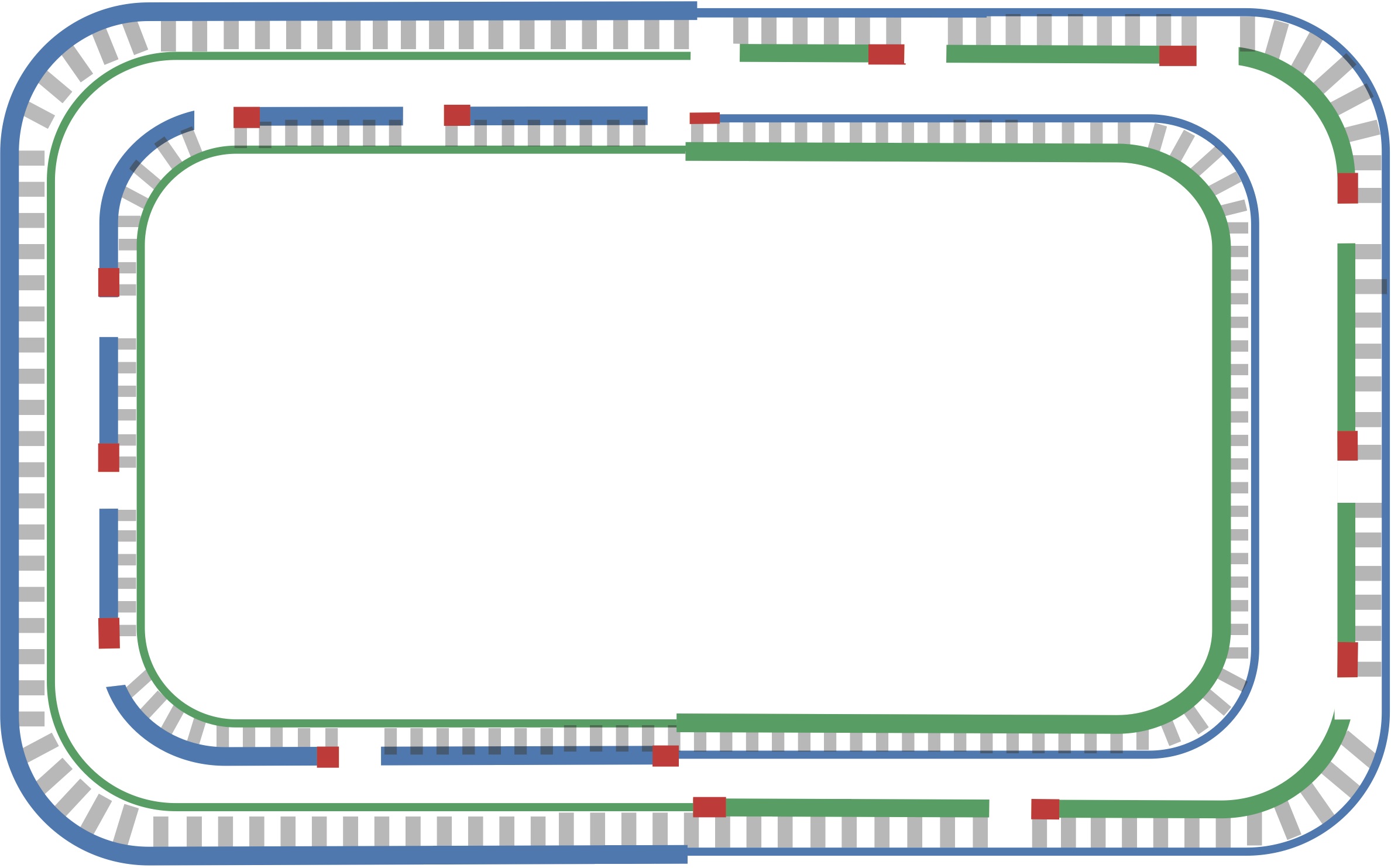
Since a DNA polymerase can only move in the reverse (3′ → 5′) direction, it can copy nucleotides non-stop from ori to ter along leading half-strands. However, replication on lagging half-strands is very different because a DNA polymerase cannot move in the forward (5′ → 3′) direction; on these half-strands, a DNA polymerase must replicate backwards toward ori. Take a look at the figure below to see why this must be the case.

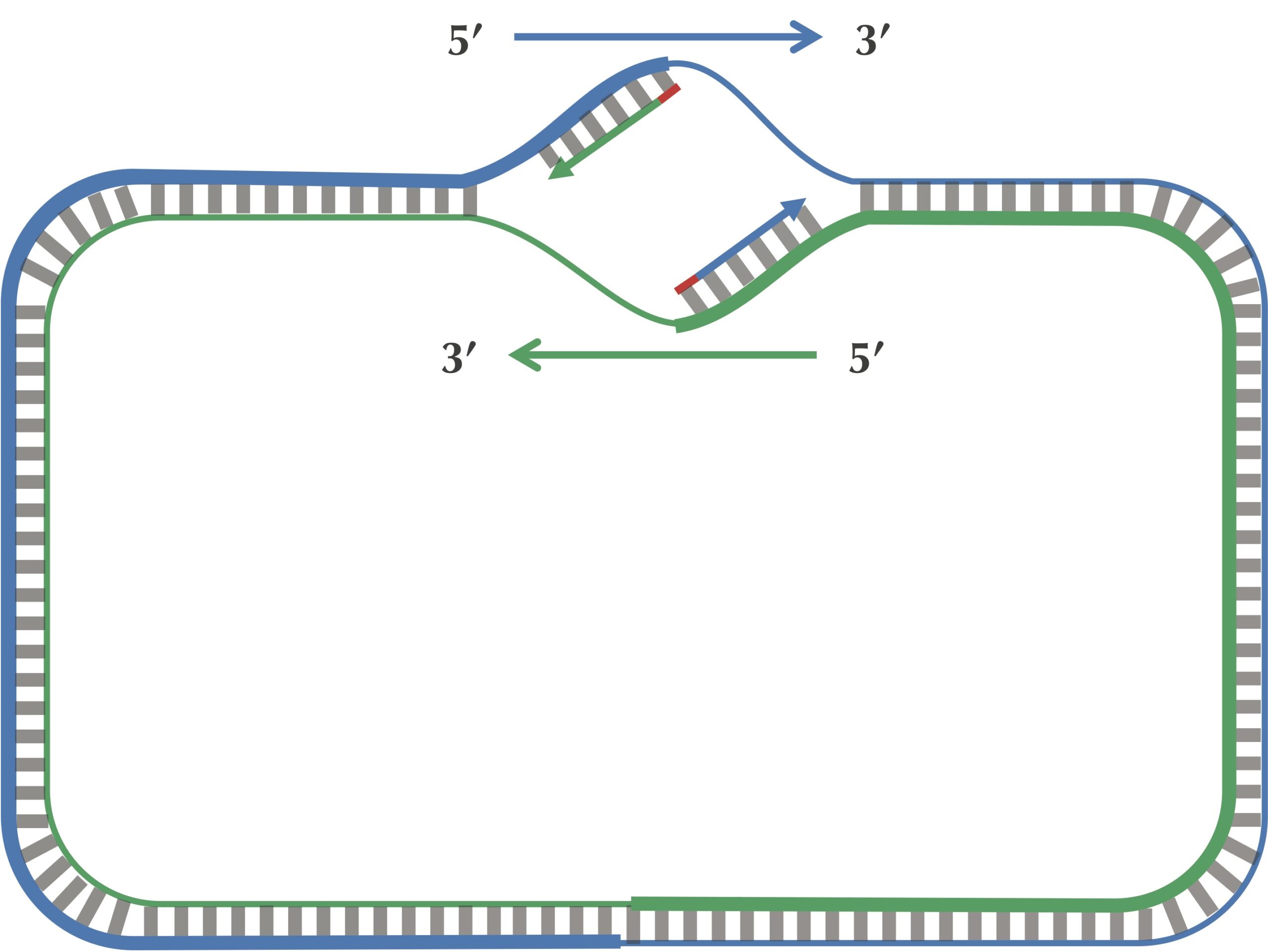
Replication begins at *ori* (primers shown in red) with the synthesis of fragments on the leading half-strands (shown by thick lines). A DNA polymerase must wait until the replication fork has opened some (small) distance before it starts copying the lagging half-strands (shown by thin lines) back toward *ori*.

On a lagging half-strand, in order to replicate DNA, a DNA polymerase must wait for the replication fork to open a little (approximately 2,000 nucleotides) until a new primer is formed at the end of the replication fork; afterwards, the DNA polymerase starts replicating a small chunk of DNA starting from this primer and moving backward in the direction of ori. When the two DNA polymerases on lagging half-strands reach ori, we have the situation shown in the figure below. Note the contrast between this figure and our original (incorrect) picture of the replication process.

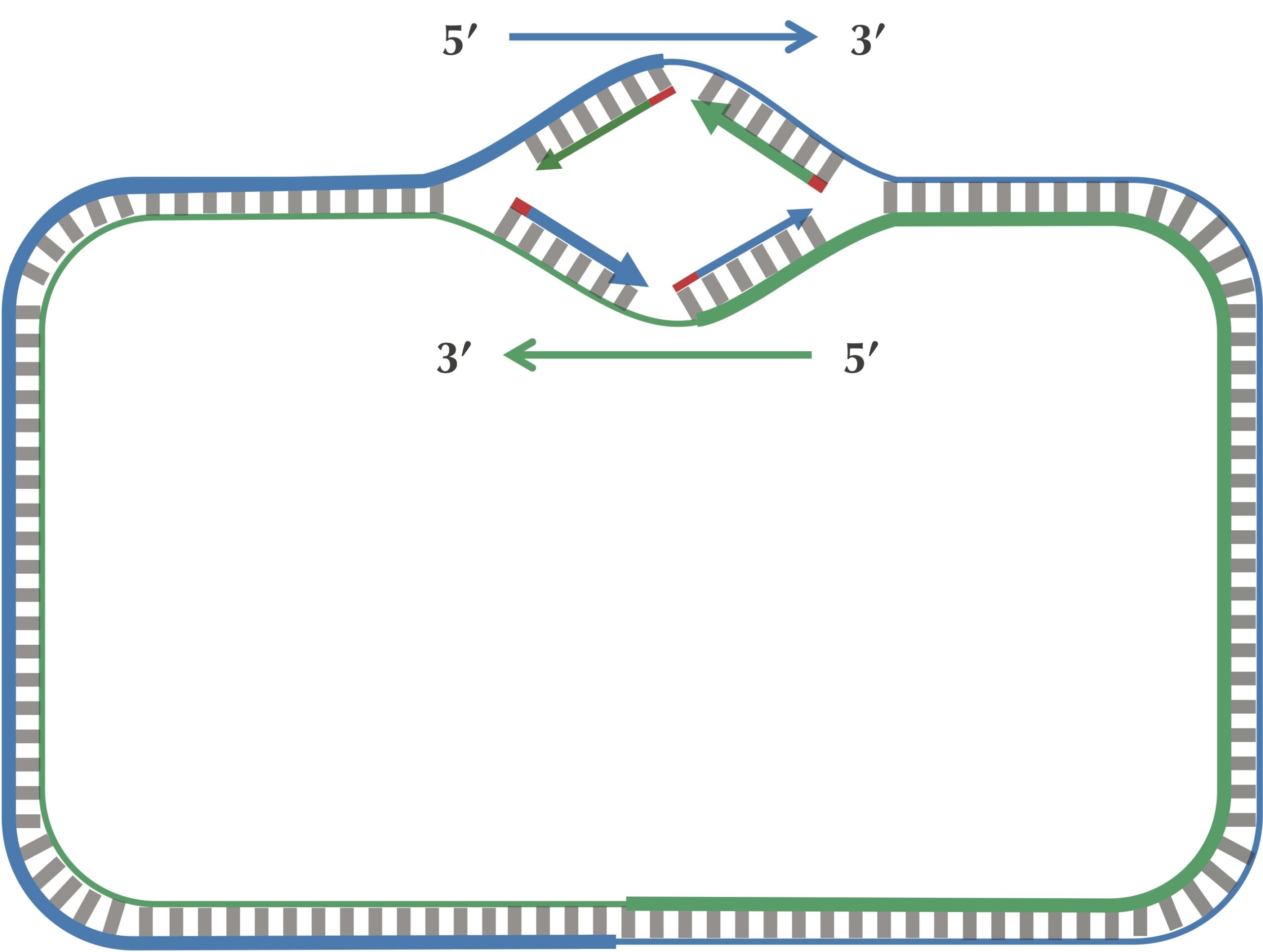
The daughter fragments are now synthesized (after some delay) on the lagging half-strands (shown by thin lines).

After this point, replication on each leading half-strand progresses continuously; however, a DNA polymerase on a lagging half-strand has no choice but to wait again until the replication fork has opened another 2,000 nucleotides or so. It then requires a new primer to begin synthesizing another fragment back toward ori. On the whole, replication on a lagging half-strand requires occasional stopping and restarting, which results in the synthesis of short Okazaki fragments that are complementary to intervals on the lagging half-strand. You can see these fragments forming in the figure below.

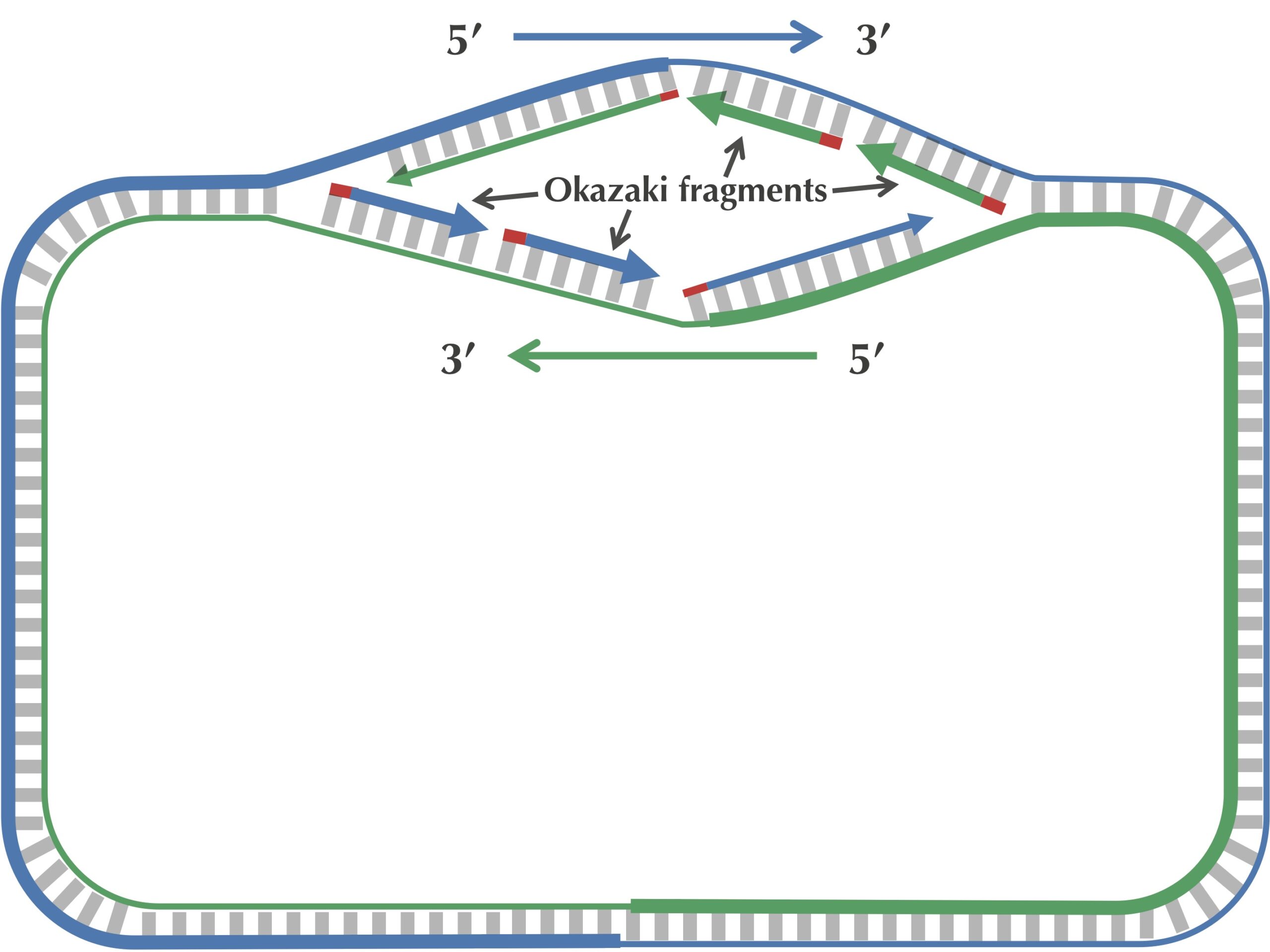
The replication fork continues growing. Only one primer is needed to replicate the leading parent half-strands (shown by thick lines), while the lagging half-strands (shown by thin lines) require multiple primers in order to synthesize Okazaki fragments. Two of these primers are shown in red on each lagging half-strand.

When the replication fork reaches ter, the replication process is almost complete, but gaps still remain between the disconnected Okazaki fragments, as shown in the figure below.

Replication is nearly complete, as all daughter DNA is synthesized. However, half of each daughter chromosome contains disconnected Okazaki fragments.

Finally, consecutive Okazaki fragments are sewn together by an enzyme called DNA ligase, resulting in two intact daughter chromosomes, each consisting of one parent strand and one newly synthesized daughter strand, as shown in the figure below. In reality, DNA ligase does not wait until after all the Okazaki fragments have been replicated to start sewing them together.

Okazaki fragments have been sewn together, resulting in two intact chromosomes.

Deamination

We have seen that as the replication fork expands, DNA polymerase synthesizes DNA quickly on the leading half-strand but suffers delays on the lagging half-strand. Notice that since the replication of a leading half-strand proceeds quickly, it lives double-stranded for most of its life. Conversely, a lagging half-strand spends a much larger amount of its life single-stranded, waiting to be used as a template for replication. This discrepancy between the leading and lagging half-strands is important because single-stranded DNA has a much higher mutation rate than double-stranded DNA. In particular, if one of the four nucleotides in single-stranded DNA has a greater tendency than other nucleotides to mutate in single-stranded DNA, then we should observe a shortage of this nucleotide on the lagging half-strand. It might also explain the strange phenomenon that we saw earlier in this section with respect to guanine and cytosine frequencies.

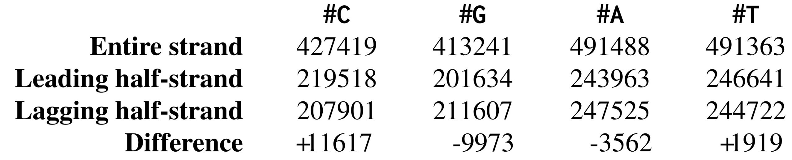
Following up on this thought, let’s examine the nucleotide counts of the leading and lagging half-strands. The nucleotide counts for Thermotoga petrophila are shown in the figure below. Although the frequencies of A and T are practically identical on the two half-strands, C is more frequent on the leading half-strand than on the lagging half-strand, resulting in a difference of 219518 − 207901 = +11617. Its complementary nucleotide G is less frequent on the leading half-strand than on the lagging half-strand, resulting in a difference of 201634 − 211607 = −9973.

Counting nucleotides in the *Thermotoga petrophila* genome on the leading and lagging half-strands.

It turns out that we observe these discrepancies because cytosine(C) has a tendency to mutate into thymine (T) through a process called deamination. Deamination rates rise 100-fold when DNA is single-stranded, which leads to a decrease in cytosine on the lagging half-strand, thus forming mismatched base pairs T-G as shown in the figure below. These mismatched pairs can further mutate into T-A pairs when the bond is repaired in the next round of replication, which accounts for the observed decrease in guanine (G) on the leading half-strand (recall that a lagging parent half-strand synthesizes a leading daughter half-strand, and vice-versa).

A mutation of a cytosine nucleotide to a thymine nucleotide on a lagging half-strand will cause DNA polymerase to pair the new thymine with an adenine, thus reducing the amount of guanine present on the leading half-strand as well in the daughter chromosome.

STOP: If deamination changes cytosine to thymine, why do you think that the lagging half-strand still has some cytosine?

Half of the daughter DNA will therefore have a shortage of C on the lagging half-strand and a shortage of G on the leading half-strand. Over time, mutations like this will build up in the population, and produce the disparities that we saw previously in the counts of cytosine and guanine on opposing half-strands.

The skew diagram

Let’s see if we can take advantage of the peculiar statistics caused by deamination to locate ori even more accurately than the approach that we illustrated previously. As the figure below shows, the difference between the total amount of guanine and the total amount of cytosine is negative on the leading half-strand (201634 − 219518 = −17884) and positive on the lagging half-strand (211607 − 207901 = 3706). Thus, our idea is to traverse the genome, keeping a running total of the difference between the counts of G and C. If this difference starts increasing, then we guess that we are on the lagging half-strand; on the other hand, if this difference starts decreasing, then we guess that we are on the leading half-strand. See the figure below.

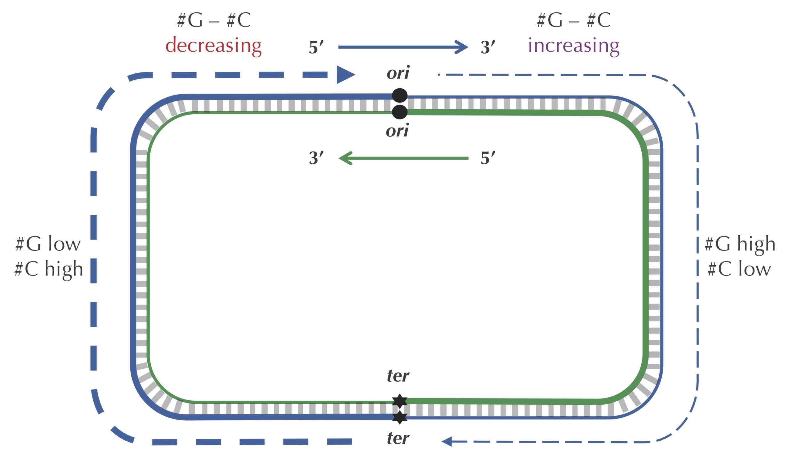
Because of deamination, each lagging half-strand has a shortage of cytosine compared to guanine, and each leading half-strand has a shortage of guanine compared to cytosine. The dashed blue line illustrates an imaginary walk along the outer strand of the genome counting the difference between the counts of guanine and cytosine. We assume that the difference between these counts is positive on the lagging half-strand and negative on the leading half-strand.

STOP: Imagine that you are reading through the genome (in the 5′ → 3′ direction) and notice that the difference between the guanine and cytosine counts just switched its behavior from decreasing to increasing. Where in the genome are you?

Since we don’t know a priori the location of ori in a circular genome, we will have a linear string genome where the position of ori is not indicated. For a genome of length n, define the skew array of genome as the array of length n+1 whose i-th value is the difference between the total number of occurrences of G and the total number of occurrences of C in the first i nucleotides of genome. This leads us to the following computational problem. You may like to practice your pseudocode skills by writing a function to solve this problem.

Skew Array Problem

Input: A DNA string genome.

Output: The skew array of genome.

We can visualize a skew array with a chart called a skew diagram. The skew diagram is a line graph that plots the number of nucleotides k encountered in genome on the x-axis, and the k-th value of the skew array on the y-axis. A skew diagram for a short DNA string is shown in the figure below.

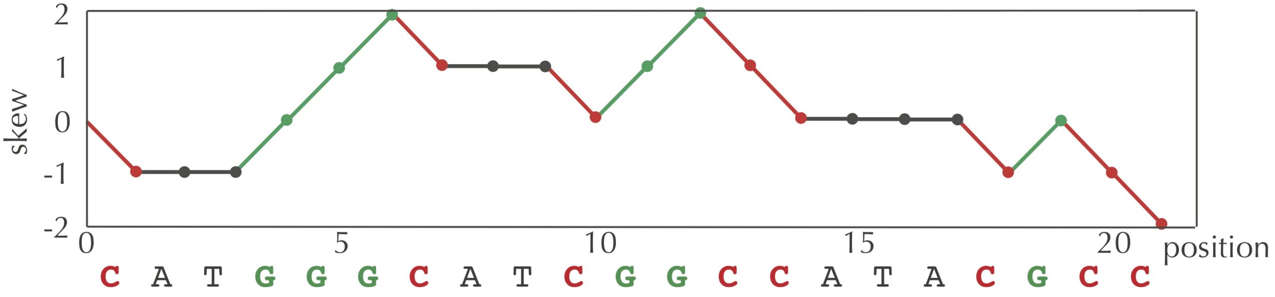
The skew diagram for *genome* = `"CATGGGCATCGGCCATACGCC"`.

The above skew diagram provides an insight, which is that the difference between the number of G and the number of C encountered in the first i nucleotides of genome differs by at most 1 from this difference when considering the first i–1 nucleotides of genome. This insight leads to a solution to the Skew Array Problem below, called SkewArray(). This function employs a subroutine Skew() that takes a symbol (A, C, G, or T) as input and returns 1 if the symbol is G, -1 if the symbol is C, and 0 otherwise.

SkewArray(genome)
    n ← length(genome)
    array ← array of length n + 1
    array[0] ← 0
    for every integer i between 1 and n
        array[i] = array[i-1] + Skew(genome[i-1])
    return array

Skew(symbol)
    if symbol = 'G'
        return 1
    else if symbol = 'C'
        return -1
    return 0

The figure below depicts the skew diagram for a linearized E. coli genome. Notice the very clear V-shaped pattern! It turns out that the skew diagram for many bacterial genomes has a similar characteristic shape.

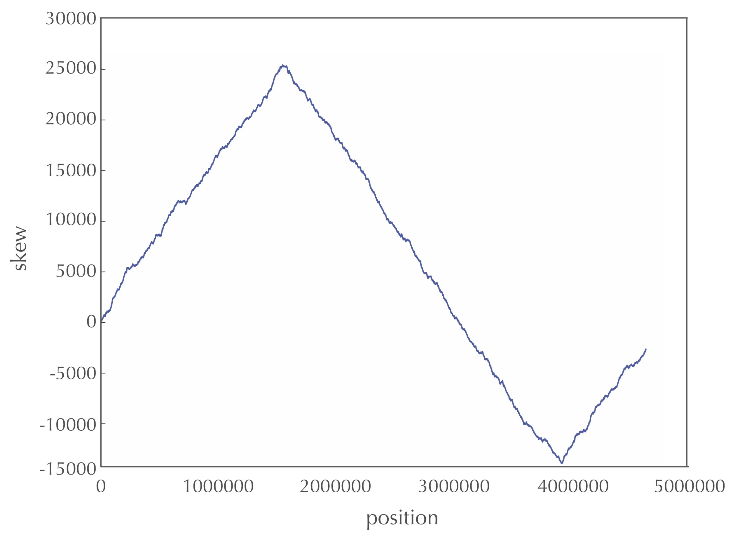
The skew diagram for *E. coli* achieves a maximum and minimum at positions 1550413 and 3923620, respectively.

STOP: After looking at the skew diagram in the figure above, where do you think that ori is located in E. coli?

Let’s follow the 5′ → 3′ direction of DNA and walk along the chromosome from ter to ori (along a leading half-strand), then continue on from ori to ter (along a lagging half-strand). We have already reasoned that the skew should generally be decreasing along the leading half-strand and increasing along the lagging half-strand. Thus, the skew should achieve a minimum at the position where the reverse half-strand ends and the forward half-strand begins, which is exactly the location of ori! We have just developed an algorithm for locating ori: it should be found where the skew attains a minimum. To be precise, we can state this as a computational problem. Again, you may want to try solving this problem before looking at our pseudocode.

Minimum Skew Problem

Input: A DNA string genome.

Output: All indices i of the skew array of genome achieving the minimum value in the skew array.

To solve the Minimum Skew Problem, we employ SkewArray() as a subroutine along with a subroutine MinIntegerArray() that finds the minimum value in an array of integers, which we encountered in Chapter 0.

MinimumSkew(genome)
    indices ← array of integers of length 0
    n ← length(genome)
    array ← SkewArray(genome)
    m ← MinIntegerArray(array)
    for every integer i between 0 and n
        if array[i] = m
            indices = append(indices, i)
    return indices

STOP: Note that the skew diagram changes depending on where we start our walk along the circular chromosome. Do you think that the minimum of the skew diagram points to the same position in the genome regardless of where we begin walking to generate the skew diagram?

Next lesson