A cellular automaton is a grid of (typically square) cells, along with a collection of clearly defined rules that allow the cells to change from one state to another. An automaton has finitely many states, and the rules for a cell changing from one state to another are based only on the cell’s current state and the states of the cells in their immediate surroundings. We would never mistake such a system for an intelligent one.
Our goal in this chapter is to build a cellular automaton that can display self-replication. Yet we will begin by illustrating how cellular automata work by considering a simpler cellular automaton devised in 1970 by John Conway called the Game of Life. Conway was a prolific mathematician who was also largely responsible for popularizing the “Doomsday Algorithm” that we previously described to derive the day of the week corresponding to a given date.
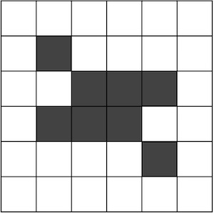
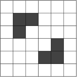
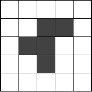
Each cell of the two-dimensional grid in the Game of Life has one of two states: alive (black) and dead (white). A sample two-state cellular automaton is shown in the figure below.
Figure: A sample two-state cellular automaton. Black cells are in one state, which we think of as alive, and white cells are in the other state, which we think of as dead.
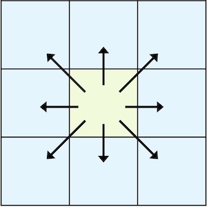
A cellular automaton also includes rules describing how cells can change states from one generation to the next. We first define the Moore neighborhood of a cell as the eight cells that border either an edge or a corner of a given cell (see figure below).
Figure: A cell (shown in green) along with the eight cells forming its Moore neighborhood (shown in blue).
The five Game of Life rules dictating state changes from one generation of the automaton to the next are summarized as follows. These rules are deterministic; that is, they are universal across the entire grid of cells and are always applied consistently.
A: If a cell is alive and has either two or three live neighbors, then it remains alive.
B: If a cell is alive and has zero or one live neighbors, then it dies out.
C: If a cell is alive and has four or more live neighbors, then it dies out.
D: If a cell is dead and has more than or fewer than three live neighbors, then it remains dead.
E: If a cell is dead and has exactly three live neighbors, then it becomes alive.
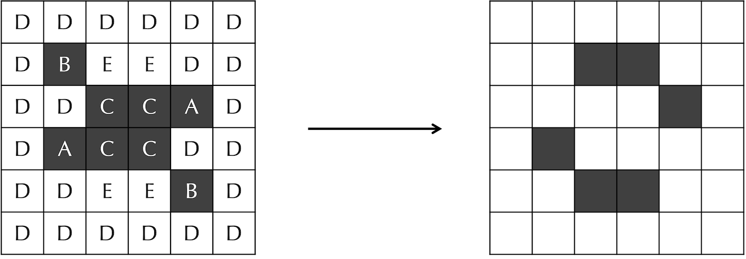
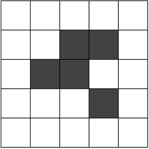
In the figure below on the left, we label each cell in the automaton previously considered with “A”, “B”, “C”, “D”, or “E”, according to which of the above five rules if falls under. We then apply these rules to produce the next generation of this board, shown on the right.
Figure: A sample Game of Life board (left) along with its updated board after one generation (right). We label each cell in the board on the left with the rule label that applies to it when updating that cell. We assume that the board stretches infinitely in every direction and that all cells beyond the boundaries shown are dead.
Exercise: Find the next generation of the Game of Life board on the right in the figure above.
Despite the simplicity of the Game of Life rules, we might apply a loose biological meaning to each of them. We could call rule A “Propagation”, since it allows life to continue in the next generation if it has enough suitable mates nearby. We could call rules B and C “Lack of mates” and “Overpopulation”, respectively, since the cell will die out if it has too few or too many neighbors. And we could call rule D “Rest in peace”, since in most cases dead cells will not spontaneously regenerate.
Were the Game of Life confined to these four rules, then the number of live cells could never increase, since any time that a cell died, there would be no way for it to come back alive. Staggering to the rescue is the beautiful rule E, which we call “Zombie”, as it allows a cell to arise from the dead if it has exactly three live neighbors.
Even with our corny biological interpretations, you may be wondering why the Game of Life applies this particular set of rules. Why should the “Propagation” step demand exactly two or three live neighbors? Why not one or two live neighbors? Or two, three, or four live neighbors? What makes these rules interesting?
Stable forms and oscillators
Most of the different sets of rules for two-state cellular automata produce boring results. Either the live cells die out quickly, or they propagate outward rapidly.
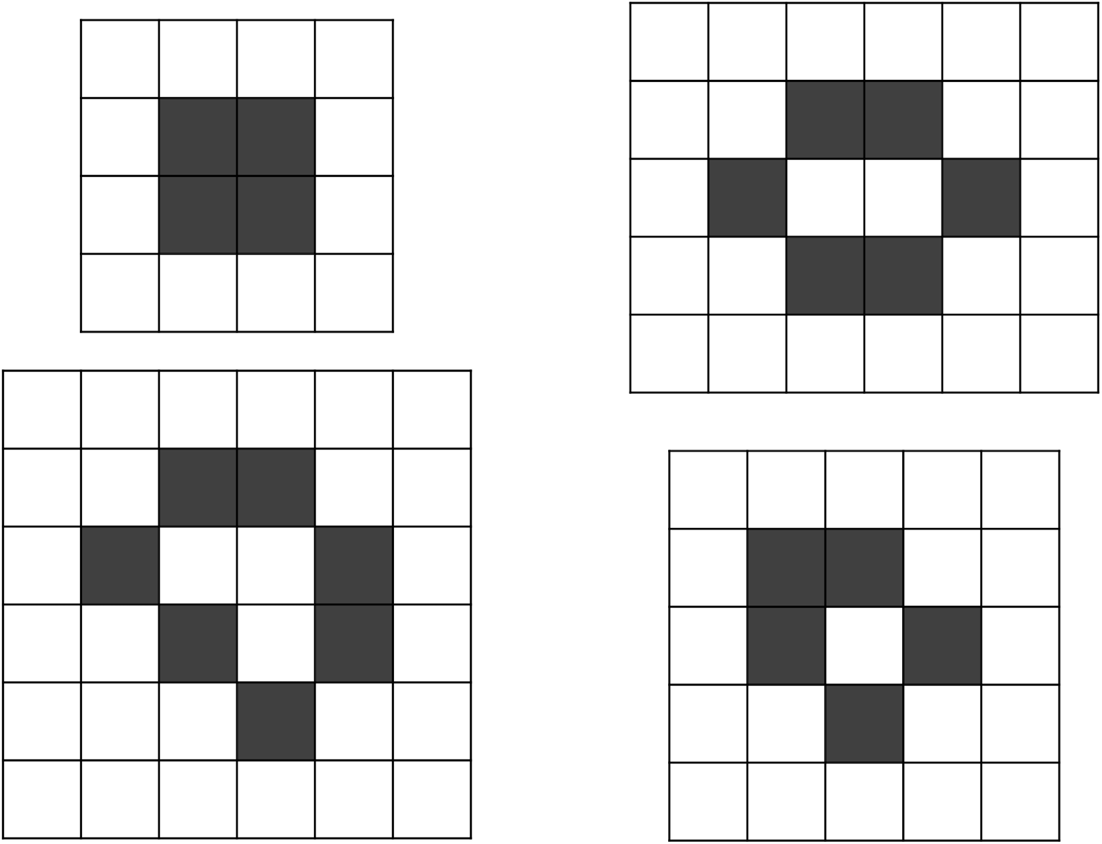
Some of the initial configurations of the Game of Life are just as predictable. The figure below shows a few stable forms (also known as still lifes), patterns whose cells’ states will not change from one generation to the next. You might wish to verify that every alive cell belongs to rule A, and every dead cell belongs to rule D.
Figure: Four stable forms in the Game of Life (there are many more). Stable forms do not change from one generation to the next. These stable forms assume that the cells surrounding the board are dead and do not change.
Exercise: Carry out the next few generations of the board below. What happens?
The animation below shows three oscillators, or patterns that after a certain number of generations repeat to their original configuration. The period of an oscillator is the number of generations that it takes for the pattern to repeat. (Where have we seen the term “period” before?) The oscillators below have period equal to 2; we will also say that stable forms are oscillators that have period equal to 1.
Figure: Three oscillating patterns with period equal to 2.
Below is a more complicated pattern called the “dinner table”, which has period 12. In December 2023, researchers proved that every positive integer is the period of some Game of Life oscillator.
Figure: The “dinner table” oscillator with period equal to 12.
The curious case of the R pentomino
Most simple patterns for the Game of Life either “die out” or eventually produce an oscillator. Perhaps the Game of Life would have been just a quirky novelty were it not for the curious case of two simple five-cell patterns. The first is called a glider, shown in the figure below.
Figure: A five-cell glider pattern.
When we animate the glider, what appears to be a swimming five-cell automaton emerges, shown in the animation below. Without outside interference, a glider is immortal, swimming off into infinity.
Figure: A lone glider, animated over 50 generations. Look at the little guy go.
The second five-cell pattern of interest is the R pentomino, shown in the figure below. Note that the R pentomino is very similar to the glider, formed by moving only a single live cell by one unit left.
Figure: The R pentomino consists of five alive cells in the above configuration that resembles a lower case “r”.
Animating the R pentomino provides a surprise, shown in the animation below. Over a thousand generations, the interior of the automaton converges to a collection of stable forms and oscillators of period 2. However, in the meantime, six gliders are formed (five early on and one toward the end of the animation). How can something so beautiful and complex derive from five simple rules?
Figure: The R pentomino animated over 1,200 generations. Five gliders are produced early on, and after several hundred additional generations, a sixth glider is produced. At this point, the board converges to a state of stable forms and period-2 oscillators.
Gosper’s gun
The R pentomino is interesting, but the growth of the population of live cells for this pattern is eventually confined to the oscillators and the six gliders that are eventually produced. Can an automaton’s population grow infinitely large?
This question remained unresolved until 1970, when Bill Gosper found the following pattern named the Gosper glider gun.
Figure: The initial Gosper glider gun, which consists of 36 live cells.
When we animate Gosper’s pattern, it looks as if the two sides of the pattern are communicating in an effort to fire off gliders (see below). As the number of generations increases, the number of gliders grows without bound.
Figure: An animation of Gosper’s gun showing the production of infinitely many gliders, meaning that the population of live cells grows without bound. (Some of the gliders fly off the visible board).
Note: You might have noticed that Gosper’s gun represents the header image of this chapter, except that we have rendered cells as circles and switched the colors for alive and dark cells. If you like how this looks, keep reading! We will generate this image in the chapter’s code alongs.
The Game of Life Problem and the case for planning
Although many more amazing patterns have been discovered for the Game of Life, none of these patterns exhibits von Neumann’s desired principle of self-replication. Returning to our robotics analogy, let us think of a Gosper gun as a factory that produces gliders one at a time. If the gliders instead could then produce copies of themselves, then the gliders would grow not just infinitely but exponentially, just like real cells.
We will place our search for a self-replicating cellular automaton on hold for the current time, since we have much to learn in order to implement the Game of Life. We state our work as a computational problem below.
Game of Life Problem
Input: An initial configuration of the Game of Life board initialBoard, and an integer numGens.
Output: All numGens + 1 configurations of this board over numGens generations of the Game of Life, starting with initialBoard.
You may be familiar with the Hollywood trope of a hacker who enthusiastically saves the day by hammering away at a keyboard at 100 words per minute. In practice, starting with coding is the last thing that we should do when presented with a challenging computational problem; the programmer’s most powerful tool is not the keyboard but the pencil.
As for us, if we try to organize hundreds of lines of code in our heads without planning in advance, we are doomed to produce buggy, poorly organized code. How, then, should we go about planning to solve a computational problem like the Game of Life Problem?