Setup
Note: These exercises are similar to the first module in my free online course Biological Modeling. If you enjoy these exercises, I think you’ll love Biological Modeling too. You can check it out at biologicalmodeling.org. There’s even an E-book and a print book! If you have ever wondered how your cells can quickly react to their environment and perform complex tasks without intelligence, why the original SARS coronavirus fizzled out but SARS-CoV-2 spread like wildfire around the planet, or how algorithms can be trained to “see” cells as well as a human, then I think that you will love it.
We are providing starter code for this assignment as a compressed file grayScott.zip. Please download this file, extract it, and add it to your go/src directory. Please make sure that this folder contains the following files:
functions.go: this is where you should place the functions that you implement in this assignment.datatypes.go: do not edit this file, which contains a couple of type declarations that we will explain soon.drawing.go: do not edit this file, which contains functions similar to those used for drawing automata that we will use for drawing our simulation.main.go:after we implement all functions necessary for our simulation, we will edit this file to run our simulation.
You should also ensure that, from following the code-along, that you have "github.com/llgcode/draw2d", "canvas", and "gifhelper" folders within "go/src".
Finally, from following our work on visualizing a skew array, you should already have plotting code in go/src/gonum.org/v1/plot/. Please ensure that this code exists, and in particular, ensure that you have code in your go/src/gonum.org/v1/plot/palette/moreland directory, which we will use in order to color cells in our automaton.
Check your work with our autograders
If you are logged in to our course on Cogniterra, then you can find the practice problems for this chapter linked in the window below, where you can enter your code into our autograders and get real time feedback. You can also view these exercises using a direct link. Beneath this window, we provide a full description of all this chapter’s exercises.
An Introduction to Turing Patterns and Reaction-Diffusion
In 1952, two years before his untimely demise, Alan Turing published his only paper on biochemistry, in which he asked: “Why do zebras have stripes?” Turing was not asking why zebras have evolved to have stripes — this question was unsolved in his time, and recent research has indicated that the stripes may be helpful in warding off flies. Rather, Turing was interested in what biochemical mechanism could produce the stripes that we see on a zebra’s coat. And he reasoned that some limited set of molecular “rules” could cause stripes to appear on a zebra’s coat.
Turing’s insight was that remarkable high-level patterns could arise if we combine particles diffusing randomly with chemical reactions, in which colliding particles interact with each other. Such a model is called a reaction-diffusion system, and the emergent patterns are called Turing patterns in his honor.
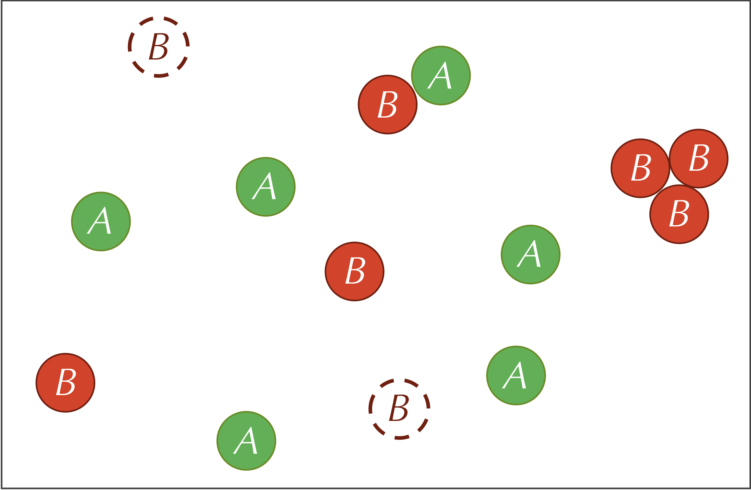
We will consider a reaction-diffusion system having two types of particles, A and B. The system is not explicitly a predator-prey relationship, but you may like to think of the A particles as prey and the B particles as predators for reasons that will become clear soon.
Both types of particles diffuse randomly through two-dimensional space, but the A particles diffuse more quickly than the B particles, meaning that they move farther in a single unit of time. (One common assumption is that A particles diffuse twice as quickly as B particles.)
The system that we will consider will have three reactions. First, A particles are added into the system at some constant feed rate f. As a result of the feed reaction, the concentration of the A particles increases by a constant number in each time step.
Second, B particles are removed from the system at a constant kill rate k. As a result of the kill reaction, the number of B particles in the system will decrease by a factor of k in a given time step. That is, the more B particles that are present, the more B particles will be removed.
Third, our reaction-diffusion system includes the following reaction involving both particle types. The particles on the left side of this reaction are called reactants, and the particles on the right side are called products.
A + 2B → 3B
That is, if an A particle and two B particles collide with each other, then the A particle has some fixed probability of being replaced by a third B particle. This probability could vary based on the presence of a catalyst and the orientation of the particles, and it directly relates to the rate at which this reaction occurs. This third reaction is why we compared A particles to prey and B particles to predators, since we may like to conceptualize the reaction as two B particles consuming an A particle and producing an offspring B particle.
The three reactions defining our system are summarized by the figure below.

A parameter is a variable quantity used as input to a model. Parameters are inevitable in biological modeling (and data science in general), and as we will see, changing parameters can cause major changes in the behavior of a system.
Five parameters are relevant to our reaction-diffusion system: the feed rate (f) of A particles, the kill rate k of the B particles, the predator-prey reaction rate (r), and the diffusion rates (dA and dB , respectively) of the A and B particles.
We think of all these parameters as dials that we can turn, observing how the system changes as a result. For example, if we raise the diffusion rate, then the particles will be moving around and colliding with each other more, which means that we will see more of the reaction A + 2B → 3B.
Modeling the Diffusion of a Single Particle with an Automaton
From a particle simulator to an automaton
One way to simulate our system would be to represent each particle as a point in two-dimensional space and then simulate each point individually as it randomly moves. When two B particles collide with an A particle, we could relabel the A particle as a B particle.
However, building such a simulation would require an enormous amount of computational resources to track each particle, to determine when particles are nearby, and to recompute velocities of points every time that they collide.
Our goal is to move from a “fine-grained” model such as this one to a more “coarse-grained” model that will allow us to appreciate Turing patterns without the computational overhead required to track particles. To do so, we will grid off two-dimensional space into cells and store only the concentration of each type of particle found inside the cell. We will typically use initial values for these concentrations that lie between 0 and 1.
We hope that our idea of gridding off space into cells sounds familiar, since the model that we are building is another form of a cellular automaton! Furthermore, just as we have seen throughout this chapter, we will represent diffusion by exchanging particle concentrations of a cell and its (Moore) neighbors.
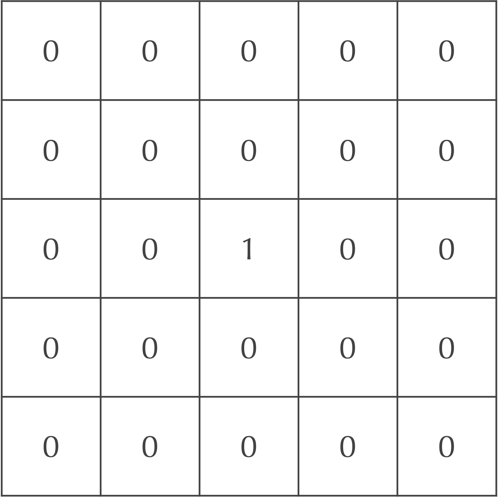
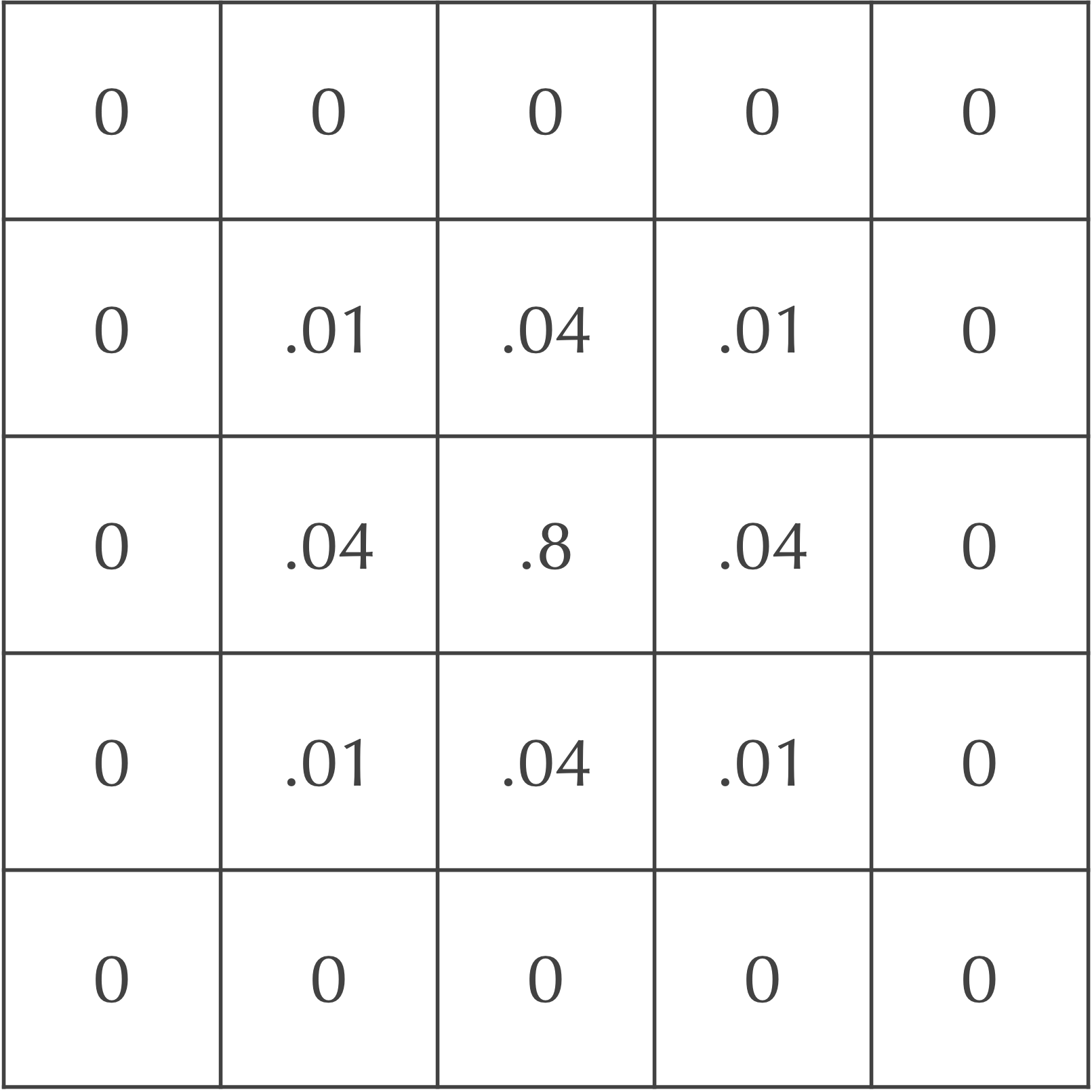
We will demonstrate how diffusion works using an example that includes A particles; we will later add B particles as well as reactions to our model. Say that the particles are at maximum concentration in the central cell of our grid and are present nowhere else, as shown in the figure below.
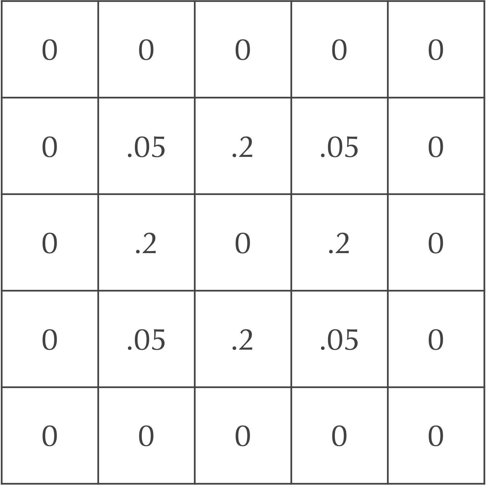
We will now update the grid of cells after one time step to mimic particle diffusion. To do so, we will spread out the concentration of particles in each square to its eight neighbors. For example, we could assume that 20% of the current cell’s concentration diffuses to each of its four adjacent neighbors, and that 5% of the cell’s concentration diffuses to its four diagonal neighbors. Because the central square in our ongoing example is the only cell with any particles, the updated concentrations after a single time step are shown in the following figure.
After an additional time step, the particles continue to diffuse outward. For example, consider again the board after a single time step, shown above.
Each diagonal neighbor of the central cell in the above figure, which has a concentration of 0.05 after one time step, will lose all of its particles in the following step. Each of these cells will also gain 20% of the particles from two of its adjacent neighbors, along with 5% of the particles from the central square (which doesn’t have any particles). This makes the updated concentration of this cell after two time steps equal to 2(0.2)(0.2) + 0.05(0) = 0.08.
The four cells directly adjacent to the central square, which have a concentration of 0.2 after one time step, will also gain particles from their neighbors. Each such cell will receive 20% of the particles from two of its adjacent neighbors and 5% of the particles from two of its diagonal neighbors, which have a concentration of 0.2. Therefore, the updated concentration of each of these cells after two time steps is 2(0.2)(0.05) + 2(0.05)(0.2) = 0.02 + 0.02 = 0.04.
Finally, the central square has no particles after one step, but it will receive 20% of the particles from each of its four adjacent neighbors, as well as 5% of the particles from each of its four diagonal neighbors. As a result, the central square’s concentration after two time steps is 4(0.2)(0.2) + 4(0.05)(0.05) = 0.16 + 0.01 = 0.17.
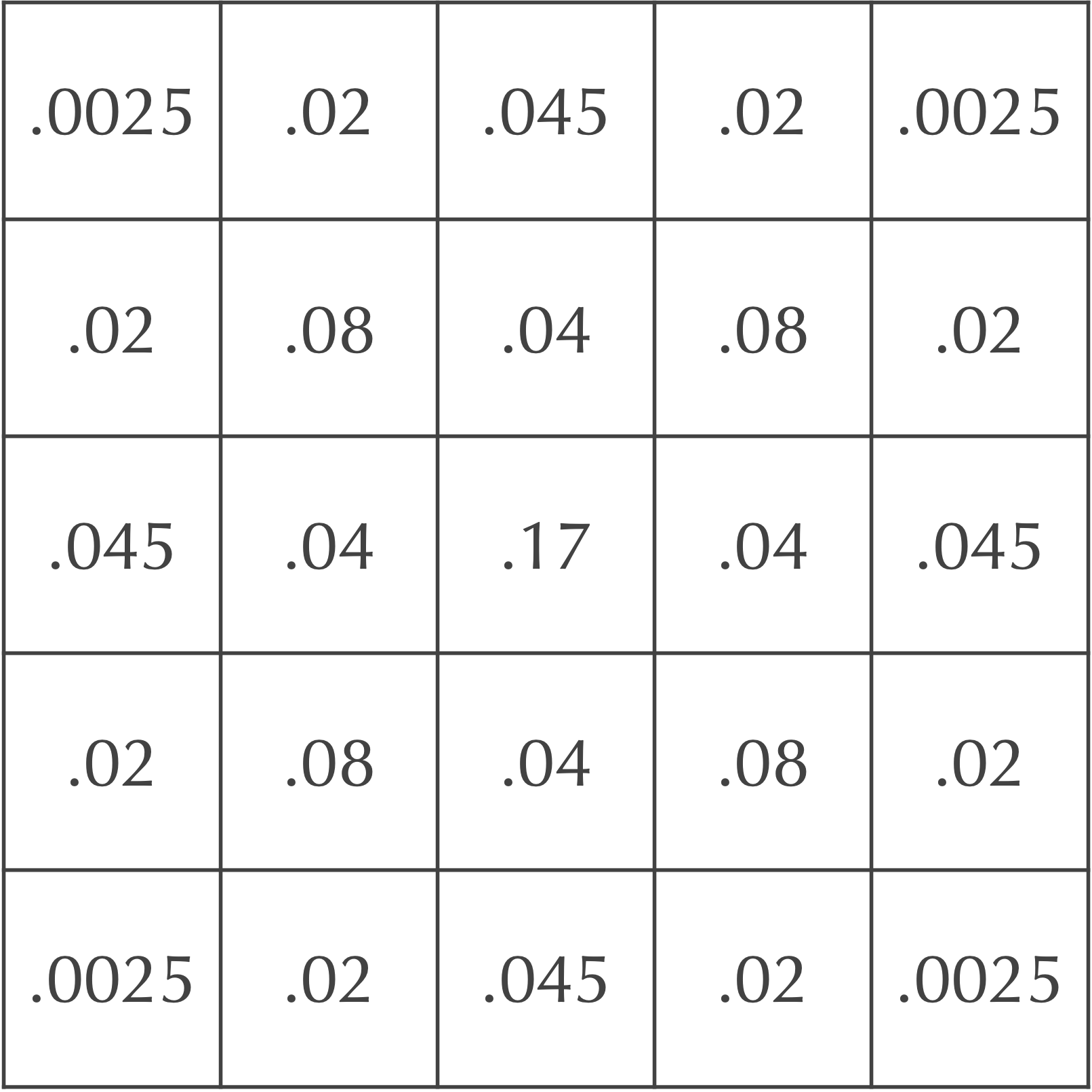
In summary, the central nine squares after two time steps are as shown in the following figure.
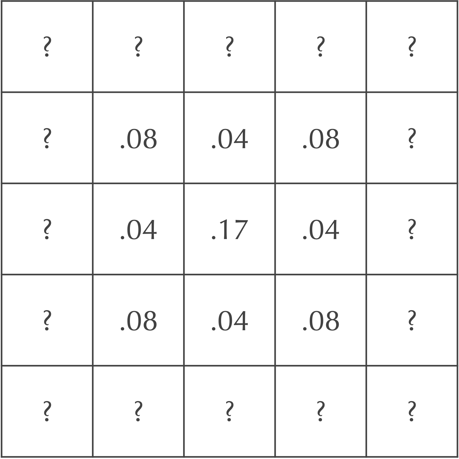
Exercise: Fill in the value of each of the cells labeled “?” by hand.
Matrix convolutions and diffusion
We should pause to make our model of diffusion a bit more formal, and to describe what should happen now that we have cells with nonzero concentrations at the boundary of the grid, since they will lose some of their concentration over the side of the grid.
First, the diffusion process that we have been modeling is based on a matrix operation called a convolution. The convolution lends its name to the popular “convolutional neural networks” that are used for a variety of purposes including image detection.
The convolution of two m × n matrices is formed by taking the weighted sum of corresponding elements. For example, if our matrices are the 2 × 2 matrices shown below.
\begin{matrix} a & b\\ c & d \end{matrix}~~~~~~~~~~~~~~~~~~\begin{matrix} w & x\\y & z\end{matrix}The convolution of these two matrices is the weighted sum a · w + b · x + c · y + d · z.
Note: For technical reasons, mathematicians often define a convolution by flipping the rows and columns of the first matrix before taking this weighted sum. We will proceed using the definition provided above.
In practice, we commonly take the convolution of the same matrix with a variety of different matrices; the matrix that is fixed is called a kernel. For example, we have been using the following kernel without realizing it:
\begin{matrix} 0.05 & 0.2 & 0.05\\ 0.2 & -1 & 0.2\\ 0.05 & 0.2 & 0.05\\ \end{matrix}To diffuse the value at row i and column j of our grid of cells, we consider the 3 × 3 matrix formed by the cell and its Moore neighborhood, which we convolve with the above kernel. The resulting average becomes the change in the concentration of a particle in the cell at row i and column j.
An example should help make this idea clear, so consider once again our grid after a single time step, shown below.
The cell at row 1 and column 2 has the following Moore neighborhood:
\begin{matrix} 0 & 0 & 0\\ 0.05 & 0.2 & 0.05\\ 0.2 & 0 & 0.2\\ \end{matrix}When we convolve this matrix with the kernel above, we obtain the weighted sum
0.05 · 0 + 0.2 · 0 + 0.05 · 0 + 0.2 · 0.05 + (-1) · 0.2 + 0.2 · 0.05 + 0.05 · 0.2 + 0.2 · 0 + 0.05 · 0.2 = 0.01 – 0.2 + 0.01 + 0.01 + 0.01 = -0.16,
which represents the change in the cell at row 1 and column 2 due to diffusion. Therefore, if we add this value to the current value in the cell at row 1 and column 2, then we obtain 0.2 + (-0.16) = 0.04, which is the value that we found before for this cell in the next time step, as shown in the complete grid for the next time step, shown below.
Reformulating the automaton’s diffusion process as a matrix convolution applied over all cells of the grid allows us to understand what should happen at boundaries.
Consider again our grid of cells after two time steps in the figure above. If we would like to determine the updated value for the cell at row 0 and column 1, which is currently equal to 0.02, then we assume that any cells that would be considered as part of the Moore neighborhood of this cell but are not on the grid have a concentration equal to zero. In other words, when we perform the convolution, we only take the weighted sum of cells that are found within the grid. As a result, some of the concentration from the cell at row 0 and column 1 is effectively “lost” over the side of the board to neighbors above this cell that do not exist and have permanent zero concentration.
As a result, when we perform the convolution of this cell, we obtain the weighted sum
0.05 · 0 + 0.2 · 0 + 0.05 · 0 + 0.2 · 0.0025 + (-1) · 0.02 + 0.2 · 0.045 + 0.05 · 0.02 + 0.08 · 0.2 + 0.05 · 0.04 = 0.0085,
so that this cell in the next time step has concentration equal to 0.02 + 0.0085 = 0.0285.
Exercise: Use the above board to determine the concentration in the next time step for the cell at row 0 and column 0, which currently has concentration equal to 0.0025. (Hint: this cell only has three of eight Moore neighbors that lie in the grid.)
Implementing our diffusion automaton
We have used a specific 3 × 3 kernel in our examples, which is typically what we will use in practice. However, we could obtain different diffusion processes if we were to use different kernels. For example, if we wanted to spread particles only to a cell’s von Neumann neighborhood instead of its Moore neighborhood, then we might use the kernel below.
\begin{matrix} 0 & 0.25 & 0\\ 0.25 & -1 & 0.25\\ 0 & 0.25 & 0\\ \end{matrix}Whatever kernel we use, we will demand that its values sum to zero, which will ensure that (other than particles falling off the sides of the grid) the sum of all cells’ concentrations stays the same from one time step to the next. In other words, the kernel’s values summing to zero ensures that we follow the law of conservation of mass.
We are now ready to implement our automaton simulating diffusion of a single particle as a warmup exercise before we add a second particle and reactions to our model.
Code Challenge: Implement a functionDiffuseBoardOneParticle(currentBoard, kernel).
Input: A two-dimensional array of decimal numberscurrentBoardand a 3 × 3 matrix of decimal numberskernel.
Output: A two-dimensional array of decimal numbersnewBoardcorresponding to applying one time step of diffusion tocurrentBoardusing the kernelkernel.
Hint: You may want to write a couple of subroutines to help you with this code challenge. In particular, we suggest modifying our InField() function from the code along into a function InField(currentBoard, row, col) that takes a two-dimensional slice of decimal numbers currentBoard, as well as integers row and col as input. This function should return true if b[row][col] is in range, and this function should return false otherwise.
Slowing down the diffusion rate
There is just one problem: our diffusion model is too volatile! The figure below shows the initial automaton as well as its updates after each of two time steps. In a true diffusion process, all of the particles would not rush out of the central square in a single time step, only for some of them to return in the next time step.
Our solution is to slow down the diffusion process by adding a parameter dA between 0 and 1 that represents the rate of diffusion of A particles. Instead of moving a cell’s entire concentration of particles to its neighbors in a single time step, we move only a fraction dA of them.
Let us revisit our original grid, reproduced below.
Say that dA is equal to 0.2. After the first time step, only 20% of the central cell’s particles will be spread to its neighbors. Of these particles, 5% will be spread to diagonal neighbors, and 20% will be spread to adjacent neighbors. The figure below illustrates that after one time step, the central square has concentration 0.8, its adjacent neighbors have concentration 0.2 · dA = 0.04, and its diagonal neighbors have concentration 0.05 · dA = 0.01.
If you are curious how all this works with respect to the convolution, the answer is easy! Instead of convolving a cell and its Moore neighborhood by the previous kernel, given by
\begin{matrix} 0.05 & 0.2 & 0.05\\ 0.2 & -1 & 0.2\\ 0.05 & 0.2 & 0.05\\ \end{matrix}we first multiply each element of the kernel by dA:
\begin{matrix} 0.05 \cdot d_A & 0.2 \cdot d_A & 0.05 \cdot d_A\\ 0.2 \cdot d_A & -1 \cdot d_A & 0.2 \cdot d_A\\ 0.05 \cdot d_A & 0.2 \cdot d_A & 0.05 \cdot d_A\\ \end{matrix}We then use this updated matrix as our kernel.
For example, if dA is equal to 0.2, then our kernel would become
\begin{matrix} 0.01 & 0.04 & 0.01\\ 0.04 & -0.2 & 0.04\\ 0.01 & 0.04 & 0.01\\ \end{matrix}This is the kernel that we used when updating the board shown above.
Code Challenge: Improve your implementation ofDiffuseBoardOneParticle()into a functionDiffuseBoardOneParticle(currentBoard, diffusionRate, kernel)that includes a diffusion rate parameter.
Input: A two-dimensional array of decimal numberscurrentBoardand a 3 × 3 matrix of decimal numberskernel.
Output: A two-dimensional array of decimal numbersnewBoardcorresponding to applying one time step of diffusion tocurrentBoardusing the diffusion ratediffusionRatemultiplied by the kernelkernel.
The Gray-Scott model of reaction-diffusion
Adding a second particle to our diffusion simulation
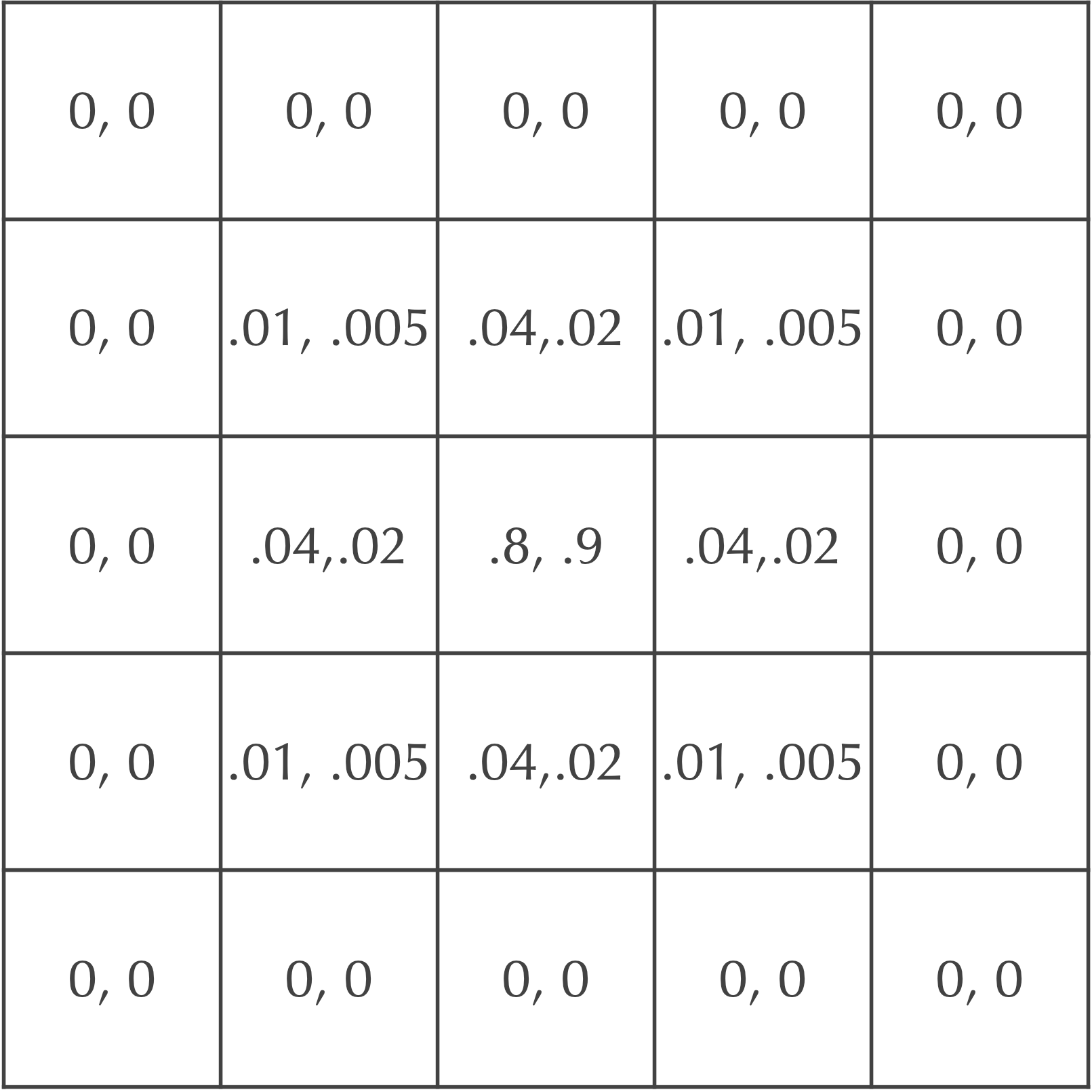
We now will add B particles to our model. In our ongoing example, we will assume that both A particles and B particles start with a concentration equal to 1 in the central square (and 0 elsewhere). Recall that when we build our reaction-diffusion simulation, we will assume that A, our “prey” molecule, diffuses twice as fast as B, the “predator” molecule. As a result, the diffusion rate dA should be equal to twice the value of dB.
For example, if we set dA equal to 0.2, then dB should be equal to 0.1. After a single time step, our cells will be updated as shown in the figure below. Each cell is labeled by an ordered pair ([A], [B]), where [A] is the concentration of A particles and [B] is the concentration of B particles.
Adding reactions to obtain the Gray-Scott model
Now that we have established a cellular automaton for coarse-grained diffusion of two particles, we will add to this model the three reactions that we introduced in the first lesson, which are reproduced below.
- A “feed” reaction in which new A particles are fed into the system at a constant rate f.
- A “death” reaction in which B particles are removed from the system at a rate k that is proportional to their current concentration.
- A “reproduction” reaction A + 2B → 3B, which takes place at some rate r.
First, we consider the feed reaction. We are tempted to simply add some constant value f to the concentration of A in each cell in each time step. However, our model will not allow the concentration of A in each cell to exceed 1, so that we will add fewer A particles for cells having high concentration of A. Specifically, if a cell has current concentration [A], then we will add f(1-[A]) to this cell’s concentration of A particles. For example, if [A] is 0.01, then we will add 0.99f to the cell because the current concentration is low. If [A] is 0.8, then we will only add 0.2f to the current concentration of A particles.
Second, we consider the death reaction of B particles, whose rate k is proportional to the current concentration of B particles. As a result, we will subtract k · [B] from the current concentration of B particles. We will often assume that k is larger than f.
Third, we have the reproduction reaction A + 2B → 3B, which takes place at a rate r. The higher the concentration of A and B, the more this reaction will take place. Furthermore, because we need two B particles in order for the collision to occur, the reaction should be even more rare if we have a low concentration of B than if we have a low concentration of A. To model this situation, if a given cell is represented by the concentrations ([A], [B]), then we will subtract r · [A] · [B]2 from the concentration of A and add r · [A] · [B]2 to the concentration of B in the next time step.
Finally, we note that the rate r of this third reaction is typically set equal to 1.
Applying diffusion with these reactions over all cells in parallel and over many generations constitutes a cellular automaton model called the Gray-Scott model, which dates from the following scientific paper. This model was not devised to produce Turing patterns, but we will see soon how Turing patterns emerge from it.
P. Gray and S.K. Scott, Autocatalytic reactions in the isothermal, continuous stirred tank reactor: isolas and other forms of multistability, Chemical Engineering Science 38 (1983) 29-43.
In summary, say that the current concentrations in a cell are given by [A] and [B], and that as the result of diffusion, the change in its concentrations are ΔA and ΔB, where a negative number represents particles leaving the cell, and a positive number represents particles entering the cell.
Then in the next time step, the particle concentrations [A]new and [B]new are given by the following equations:
[A]new = [A] + ΔA + f(1-[A]) – r · [A] · [B]2
[B]new = [B] + ΔB – k · [B] + r · [A] · [B]2 .
Before continuing, let us consider an example of how a single cell might update its concentration of both particle types as a result of reaction and diffusion. Say that we have the following hypothetical parameter values:
- dA = 0.2;
- dB = 0.1;
- f = 0.3;
- k = 0.4;
- r = 1 (the value typically used in the Gray-Scott model).
Furthermore, say that our cell has the current concentrations ([A], [B]) = (0.7, 0.5). Then as a result of diffusion, the cell’s concentration of A will decrease by 0.7 · dA = 0.14, and its concentration of B will decrease by 0.5 · dB = 0.05. It will also receive particles from neighboring cells; for example, say that it receives an increase to its concentration of A by 0.08 and an increase to its concentration of B by 0.06 as the result of diffusion from neighbors. Therefore, the net concentration changes due to diffusion are ΔA = 0.08 – 0.14 = -0.06, and ΔB = 0.06 – 0.05 = 0.01.
We will now consider the three reactions. The feed reaction will cause the cell’s concentration of A to increase by (1 – [A]) · f = 0.09. The death reaction will cause its concentration of B to decrease by k · [B] = 0.2. And the reproduction reaction will mean that the concentration of A decreases by [A] · [B]2 = 0.175, with the concentration of B increasing by the same amount.
Recall the equations that we use to update the concentration of each cell:
[A]new = [A] + ΔA + f(1-[A]) – r · [A] · [B]2
[B]new = [B] + ΔB – k · [B] + r · [A] · [B]2 .
As the result of all these processes, we update the concentrations of A and B to the following values ([A]new, [B]new) in the next time step according to the equations above:
[A]new = 0.7 – 0.06 + 0.09 – 0.175 = 0.555
[B]new = 0.5 + 0.01 – 0.2 + 0.175 = 0.485 .
We are now ready to discuss how to implement the Gray-Scott model. The question is: will we see Turing patterns?
Defining types
We begin with thinking about how we will store our data. In our cellular automaton model, each cell could be represented by a string or an integer to represent which state the cell was in.
However, this time each cell needs to store two pieces of information, corresponding to the concentrations of the two particles. We will therefore think of the board as a two-dimensional array of “cells”, each of which is just an array of length 2.
In other words, given a board b, the cell b[row][col] consists of two values: b[row][col][0] is the concentration of A particles, and b[row][col][1] is the concentration of B particles.
Planning Gray-Scott top down
Just as when building our cellular automaton model, we will plan our work with Gray-Scott top down.
It should hopefully come as no surprise that we will start with a short pseudocode function SimulateGrayScott() that takes as input an initial board, a number of generations, and the Gray-Scott parameters. This function generates a board for each generation, passing the work to a subroutine called UpdateBoard() that takes as input a single board along with all parameters and returns the board in the next generation after applying the Gray-Scott equations to each cell.
SimulateGrayScott(initialBoard, numGens, feedRate, killRate, preyDiffusionRate, predatorDiffusionRate, kernel)
	boards ← array of numGens + 1 Boards
	boards[0] ← initialBoard
	for i ← 1 to numGens
		boards[i] ← UpdateBoard(boards[i-1], feedRate, killRate, preyDiffusionRate, predatorDiffusionRate, kernel)
	return boards
We now consider UpdateBoard(). This function takes the current board along with system parameters, and it returns the board after applying all reactions over all cells.
It applies subroutines CountRows() and CountColumns() (which are analogous to functions we introduced in our cellular automaton model) as well as a subroutine InitializeBoard() that creates a board of cells and sets the concentration of both A and B particles in every cell equal to zero.
Because it is dividing the work over cells, UpdateBoard() also calls an UpdateCell() subroutine that takes as input the current board as well as a row and column index and the model parameters. UpdateCell() returns a cell (i.e., a two-dimensional array) containing the concentrations of both A and B particles in the next time step at this row and column in the grid after applying all reactions and diffusion.
UpdateBoard(currentBoard, feedRate, killRate, preyDiffusionRate, predatorDiffusionRate, kernel)
	numRows ← CountRows(currentBoard)
	numCols ← CountColumns(currentBoard)
	newBoard ← InitializeBoard(numRows, numCols)
	for row ← 0 to numRows – 1
		for col ← 0 to numCols – 1
			newBoard[row][col] ← UpdateCell(currentBoard, row, col, feedRate, killRate, preyDiffusionRate, predatorDiffusionRate, kernel)
	return newBoard
Finally, we consider UpdateCell(). This function passes all of its work to three subroutines in order to represent the Gray-Scott reactions, reproduced below.
[A]new = [A] + ΔA + f(1-[A]) – r · [A] · [B]2
[B]new = [B] + ΔB – k · [B] + r · [A] · [B]2 .
ChangeDueToDiffusion(): this function takes as input a board, row and column indices, and diffusion rates and a kernel. It returns a cell containing the change of the two particles’ concentrations in the board at the given row and column due to diffusion. We previously represented these values in the Gray-Scott equations as (ΔA, ΔB).ChangeDueToReactions(): this function takes as input a cell and the feed and kill rates. It applies the Gray-Scott reactions to the cell and returns a cell whose values represent the change in the given cell due to applying reactions. We previously represented these values in the Gray-Scott equations as (f(1-[A]) – [A] · [B]2 , – k · [B] + [A] · [B]2 ).SumCells(): we would like to add the current values in the cell to the values obtained from the previous two subroutines due to diffusion and the Gray-Scott reactions.SumCells()takes as input an arbitrary number of cells and returns a single cell whose 0-th element (corresponding to A) is formed by summing all input cells’ 0-th elements, and whose 1-th element (corresponding to B) is formed by summing all input cells’ 1-th elements.
UpdateCell(currentBoard, row, col, feedRate, killRate, preyDiffusionRate, predatorDiffusionRate, kernel)
    currentCell ← currentBoard[row][col]
    diffusionValues ← ChangeDueToDiffusion(currentBoard, row, col, preyDiffusionRate, predatorDiffusionRate, kernel)
    reactionValues ← ChangeDueToReactions(currentCell, feedRate, killRate)
    return SumCells(currentCell, diffusionValues, reactionValues)
We will leave the three subroutines in this function for you to write in pseudocode. When you have done so, we will be ready to implement all these functions and build the Gray-Scott model.
Implementing the Gray-Scott Model
Now that we have planned our code top-down, we will implement (and test) our functions bottom up. This way, we start with simpler functions.
Recall the pseudocode for UpdateCell(), which is reproduced below. We will start by implementing each of its three subroutines, beginning with SumCells().
UpdateCell(currentBoard, row, col, feedRate, killRate, preyDiffusionRate, predatorDiffusionRate, kernel)
    currentCell ← currentBoard[row][col]
    diffusionValues ← ChangeDueToDiffusion(currentBoard, row, col, preyDiffusionRate, predatorDiffusionRate, kernel)
    reactionValues ← ChangeDueToReactions(currentCell, feedRate, killRate)
    return SumCells(currentCell, diffusionValues, reactionValues)
We will first point out that we will use the following code to declare a Board and Cell type in Go. Recall that a Board is a two-dimensional array of Cell variables, and a Cell is an array of two decimals (whose first value represents the concentration of A and whose second value represents the concentration of B. This code is present in datatypes.go within the grayScott folder.
type Board [][]Cell
type Cell [2]float64
This means that whenever we encounter a Board type, we can work with it as if it were a [][]Cell, and when we encounter a Cell type, we can work with it as if it were a [2]float64
Second, we recall how variadic functions work in Go, which are functions that can take a variable number of inputs. The following function in Go takes an arbitrary number of integers as input and returns their sum. Regardless of how many integers are input into the function, they are converted into an array numbers that has scope throughout the function. This syntax will be useful when implementing SumCells().
func SumIntegers(numbers ...int) int {
	s := 0
	for _, val := range numbers {
		s += val
	}
	return s
}
Code Challenge: ImplementSumCells().
Input: an arbitrary collectioncellsofCellvariables.
Return: a singleCellvariable corresponding to summing corresponding elements in every cell incells.
We now turn to the two other subroutines of UpdateCell().
Code Challenge: Implement.ChangeDueToReactions()
Input: aCellvariablecurrentCell, and decimalsfeedRateandkillRate.
Return: aCellvariable storing the change incurrentCelldue to Gray-Scott reactions usingfeedRateas the rate of the feed reaction andkillRateas the rate of the kill reaction.
As for the diffusion subroutine, we should be able to adapt what we built before with a single particle diffusion simulator, except in this case, we are looking for the change in a cell’s concentrations due to diffusion as opposed to its updated value after diffusion.
Code Challenge: ImplementChangeDueToDiffusion().
Input: ABoardvariablecurrentBoard, integersandrow, decimal variablescolandpreyDiffusionRate, and a 3 x 3 decimal matrixpredatorDiffusionRate.kernel
Return: aCellvariable storing the result of applying diffusion reactions with parameters,preyDiffusionRate, andpredatorDiffusionRateto thekernelCellvariable atcurrentBoard[row][col].
(Note: it may be helpful to write anInField()subroutine to ensure that aCellis in range before accessing its concentrations.)
Next, we consider UpdateBoard() and UpdateCell(). Recall that the pseudocode for these two functions is found below.
UpdateBoard(currentBoard, feedRate, killRate, preyDiffusionRate, predatorDiffusionRate, kernel)
	numRows ← CountRows(currentBoard)
	numCols ← CountColumns(currentBoard)
	newBoard ← InitializeBoard(numRows, numCols)
	for row ← 0 to numRows – 1
		for col ← 0 to numCols – 1
			newBoard[row][col] ← UpdateCell(currentBoard, row, col, feedRate, killRate, preyDiffusionRate, predatorDiffusionRate, kernel)
	return newBoard

UpdateCell(currentBoard, row, col, feedRate, killRate, preyDiffusionRate, predatorDiffusionRate, kernel)
    currentCell ← currentBoard[row][col]
    diffusionValues ← ChangeDueToDiffusion(currentBoard, row, col, preyDiffusionRate, predatorDiffusionRate, kernel)
    reactionValues ← ChangeDueToReactions(currentCell, feedRate, killRate)
    return SumCells(currentCell, diffusionValues, reactionValues)
Code Challenge: Implement.UpdateBoard()
Input: ABoardvariablealong with decimalscurrentBoard,feedRate,killRate, andpreyDiffusionRate, and a 3 x 3 matrix of decimalspredatorDiffusionRate.kernel
Return: The Boardcorresponding to the next time step after applying the reaction-diffusion reactions of the Gray-Scott model tonewBoardwith the additional parameters given.currentBoard
Finally, we arrive at SimulateGrayScott(), whose pseudocode is reproduced below.
SimulateGrayScott(initialBoard, numGens, feedRate, killRate, preyDiffusionRate, predatorDiffusionRate, kernel)
	boards ← array of numGens + 1 Boards
	boards[0] ← initialBoard
	for i ← 1 to numGens
		boards[i] ← UpdateBoard(boards[i-1], feedRate, killRate, preyDiffusionRate, predatorDiffusionRate, kernel)
	return boards
Code Challenge: ImplementSimulateGrayScott().
Input: ABoardvariable, an integerinitialBoard, decimal variablesnumGens,feedRate,killRate, andpreyDiffusionRate, and a 3 x 3 decimal matrixpredatorDiffusionRate.kernel
Return: An array of+ 1 Board variablesnumGens, whereboardsisboards[0], andinitialBoardrepresents the board in the i-th time step of the Gray-Scott simulation starting withboards[i].initialBoard
Drawing Gray-Scott boards and running the simulation
Drawing Gray-Scott boards
It’s now time to put all our functions together and visualize the results of the Gray-Scott model!
First, we will explain what is contained in drawing.go, where we have two functions. The first is DrawBoards()boardsBoard variables, and two integers cellWidthnImage object for the board from the image package (we will say more about objects soon), where each cell in the grid is assigned a single color that is cellWidthcellWidth
//DrawBoards takes a slice of Board objects as input along with a cellWidth and n parameter.
//It returns a slice of images corresponding to drawing every nth board to a file,
//where each cell is cellWidth x cellWidth pixels.
func DrawBoards(boards []Board, cellWidth, n int) []image.Image {
	imageList := make([]image.Image, 0)

	// range over boards and if divisible by n, draw board and add to our list
	for i := range boards {
		if i%n == 0 {
			imageList = append(imageList, DrawBoard(boards[i], cellWidth))
		}
	}

	return imageList
}
Next, we get into the details of the DrawBoard()
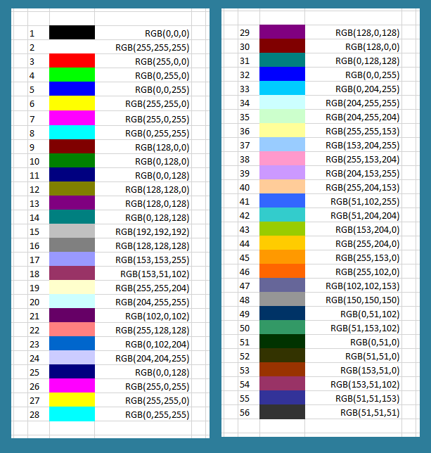
We first make an aside to discuss how your computer encodes colors. In the RGB color model, every rectangular pixel on a computer screen emits a single color formed as a mixture of differing amounts of the three primary colors of light: red, green, and blue (hence the acronym “RGB”). The amount of each primary color in a pixel is expressed as an integer between 0 and 255, inclusively, with larger integers corresponding to greater amounts of the color.
A few colors are shown in the figure below along with their RGB equivalents; for example, magenta corresponds to equal parts red and blue. Note that a color like (128, 0, 0) contains only red but appears duskier than (255, 0, 0) because the red light in that pixel has not been “turned on” fully.
We will color each cell of a Board according to its value of [B]/([A] + [B]). The expression [B]/([A] + [B]) ranges from 0 (the cell has relatively few B particles compared to A particles) to 1 (the cell has relatively many B particles compared to A particles). Therefore, we will use the color map shown below that converts decimal numbers between 0 and 1 into colors. As a result, if a cell has lots of B particles, then it will be colored closer to red, and if it has lots of A particles, then it will be colored closer to blue. This color map will be imported from the "moreland" package.
We are now ready to show the implementation of DrawBoard()bcellWidthcellWidthcellWidth
//DrawBoard takes a Board objects as input along with a cellWidth and n parameter.
//It returns an image corresponding to drawing the board to a file,
//where each cell is cellWidth x cellWidth pixels.
func DrawBoard(b Board, cellWidth int) image.Image {
    // need to know how many pixels wide and tall to make our image

    height := len(b) * cellWidth
    width := len(b[0]) * cellWidth

    // think of a canvas as a PowerPoint slide that we draw on
    c := canvas.CreateNewCanvas(width, height)

    // canvas will start as black, so we should fill in colored squares
    for i := range b {
        for j := range b[i] {
            prey := b[i][j][0]
            predator := b[i][j][1]

            // we will color each cell according to a color map.
            val := predator / (predator + prey)
            colorMap := moreland.SmoothBlueRed() // blue-red polar spectrum

            //set min and max value of color map
            colorMap.SetMin(0)
            colorMap.SetMax(1)

            //find the color associated with the value predator / (predator + prey)
            color, err := colorMap.At(val)

            if err != nil {
                panic("Error converting color!")
            }

            // draw a rectangle in right place with this color
            c.SetFillColor(color)

            x := i * cellWidth
            y := j * cellWidth
            c.ClearRect(x, y, x+cellWidth, y+cellWidth)
            c.Fill()
        }
    }

    // canvas has an image field that we should return
    return canvas.GetImage(c)
}
Running the Gray-Scott simulation
Now it comes time to run our simulation. Type the following into your main.go file. This code creates an initial board, in which the concentration of A particles is set to 1 in every cell in the grid, and the concentration of B particles is set to 0 in every cell except for a small square grid in the middle of the board, where the concentration of B particles is 1.
Run this code in the terminal by navigating to "go/src/grayScott", then typing go build and then ./GrayScott (on a Mac) or grayScott.exe (on a Windows machine). This will generate the boards of the simulation and then draw them to an animated GIF called Gray-Scott.out.gif. It may take your code a few minutes to run, but we promise that it’s worth it when it finishes.
package main

import (
	"fmt"
	"gifhelper"
)

func main() {
	numRows := 250
	numCols := 250

	initialBoard := InitializeBoard(numRows, numCols)

	frac := 0.05 // tells us what percentage of interior cells to color with predators

	// how many predator rows and columns are there?
	predRows := frac * float64(numRows)
	predCols := frac * float64(numCols)

	midRow := numRows / 2
	midCol := numCols / 2

	// a little for loop to fill predators
	for r := midRow - int(predRows/2); r < midRow+int(predRows/2); r++ {
		for c := midCol - int(predCols/2); c < midCol+int(predCols/2); c++ {
			initialBoard[r][c][1] = 1.0
		}
	}

	// make prey concentration 1 at every cell
	for i := range initialBoard {
		for j := range initialBoard[i] {
			initialBoard[i][j][0] = 1.0
		}
	}

	// let's set some parameters too
	numGens := 20000 // number of iterations
	feedRate := 0.034
	killRate := 0.095

	preyDiffusionRate := 0.2 // prey are twice as fast at running
	predatorDiffusionRate := 0.1

	// let's declare kernel
	var kernel [3][3]float64
	kernel[0][0] = .05
	kernel[0][1] = .2
	kernel[0][2] = .05
	kernel[1][0] = .2
	kernel[1][1] = -1.0
	kernel[1][2] = .2
	kernel[2][0] = .05
	kernel[2][1] = .2
	kernel[2][2] = .05

	// let's simulate Gray-Scott!
	// result will be a collection of Boards corresponding to each generation.
	boards := SimulateGrayScott(initialBoard, numGens, feedRate, killRate, preyDiffusionRate, predatorDiffusionRate, kernel)

	fmt.Println("Done with simulation!")

	// we will draw what we have generated.
	fmt.Println("Drawing boards to file.")

	//for the visualization, we are only going to draw every nth board to be more efficient
	n := 100

	cellWidth := 1 // each cell is 1 pixel

	imageList := DrawBoards(boards, cellWidth, n)
	fmt.Println("Boards drawn! Now draw GIF.")

	outFile := "Gray-Scott"
	gifhelper.ImagesToGIF(imageList, outFile) // code is given
	fmt.Println("GIF drawn!")
}
Open the GIF that you created in a browser. Isn’t it beautiful?
Rename the GIF that you just created as f_0.034_k_0.095.gif. Then, let’s run this simulation for a few different parameter values to see how the patterns that we obtain change over time. Each time, name the GIF that you produce something different.
- f = 0.034, k = 0.097
- f = 0.038, k = 0.099
- f = 0.042, k = 0.101
What do you notice?
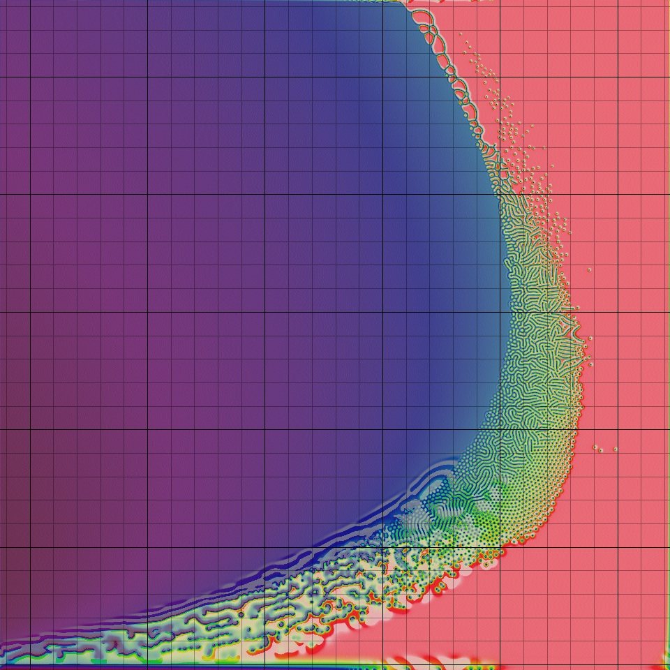
Conclusion: Turing patterns are fine-tuned
When you ran the simulation multiple times with slightly different parameters, you will have observed that the model is fine-tuned, meaning that very slight changes in parameter values can lead to significant changes in the system. These changes could convert spots to stripes, or they could influence how clearly defined the boundaries of the Turing patterns are.
The figure below shows how the Turing patterns produced by the Gray-Scott model change as the kill and feed rates vary. The square at position (x, y) shows the pattern obtained as the result of a Gray-Scott simulation with kill rate x and feed rate y. Notice how much the patterns change! In fact, the window of parameter values that produce Turing patterns is very narrow; with most parameter choices, as you may like to explore, either the A particles or the B particles win out. It makes us wonder: why should this tiny window of beauty exist?
It turns out that although Turing’s work offers a compelling argument for how zebras might have gotten their stripes, the exact mechanism causing these stripes to form is still an unresolved question. However, researchers have shown that the skin of zebrafish does exhibit Turing patterns because two types of pigment cells serve as “particles” following a reaction-diffusion model much like the one we presented in this prologue.
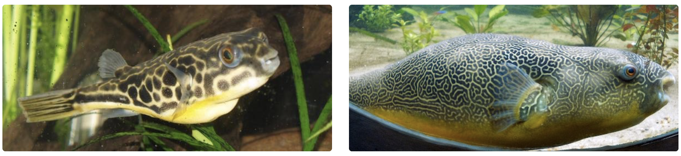
After all, take a look at the following two photos of giant pufferfish. Genetically, these fish are practically identical, but their skin patterns are very different. What may seem like a drastic change from spots to stripes is likely attributable to a small change of parameters in a fine-tuned biological system that, like much of life, is powered by randomness.
Up next
In this chapter, we started building longer programs, and we saw how we can use top-down programming to organize our work as it becomes more complex. We would also point out that by we have been able to do everything thus far in the course using a handful of basic variable types: Booleans, integers, decimals, strings, maps, and arrays.
As we work on larger and larger projects, we will see that we need to shift from working with basic types to programming objects that have attributes and can interact. For example, if we are building a gravity simulator, then we should think about a planet not as an integer, or a Boolean, but as an object that is defined by certain attributes (its size, position, current velocity, color, etc.) In the next chapter, we will start working with object-oriented programming and see how it can be used to build such a physics simulation.
Stay tuned!