Eratosthenes meets Sagan
Who first computed the circumference of the Earth? When asked this question, some students will still cheerily reply, “Christopher Columbus”! But the correct answer is Eratosthenes of Cyrene, a Greek polymath living in Alexandria, who in the 3rd Century BCE devised an ingenious experiment. No one has better explained Eratosthenes’ work than Carl Sagan, and we leave this task to him.
A trivial algorithm for finding prime numbers
Although Sagan’s story is compelling, and one that is not told often enough, the reason why we have introduced you to Eratosthenes is because of another of his interests: finding prime numbers. We remind you that an integer greater than 1 is prime if its only positive divisors are 1 and itself, and an integer greater than 1 is composite if it is not prime.
The ancient Greeks were perennially looking for order in the world around them, and yet the primes stubbornly refused to follow any discernible pattern. What is special about the number 1423 that makes it prime, while 1421 is kept out of the club?
Finding primes is a natural task to transform into a computational problem, which we state for a single input integer variable.
Prime Number Problem
Input: An integer p.
Output: “Yes” if p is prime, and “no” otherwise.
The Prime Number Problem is an example of a decision problem, a computational problem that always outputs “yes” or “no”. These problems may seem simple, but we will see much later in this work that they lie at the dark and mysterious heart of computer science.
For now, we will use the keywords truefalsetruefalse
The following pseudocode uses the truefalsep is less than 2 so that we don’t accidentally return that 0 or 1 is prime.
IsPrime(p)
    if p < 2
        return false
    for every integer k between 2 and p − 1
        if k is a divisor of p
            return false
    return true
STOP: Change the first line ofto the following:IsPrime(). How would this change the output offor every integer k between 1 and p − 1? What if we instead change this line toIsPrime()?for every integer k between 2 and p
By running IsPrime() for larger and larger input values, we can find as many primes as we like (see table below). However, this method would certainly be called the trivial algorithm for finding primes. Can we find a nontrivial algorithm to find primes faster?

One way to improve the trivial prime-finding algorithm is to make a tweak to IsPrime()false
    for every integer k between 2 and p − 1
        if k is a divisor of p
            return false
As a result, we don’t need to consider all possible divisors k of p up to p − 1; it suffices to stop at √p, and we can therefore revise IsPrime()
IsPrime(p)
    for every integer k between 2 and √p
        if k is a divisor of p
            return false
    return true
This insight has helped us speed up our approach, but Eratosthenes’ idea was more clever. Yet before we describe his algorithm, which we will recklessly call “the world’s second nontrivial algorithm”, we will first ask ourselves how we know that the prime numbers go on forever. After all, if it were true that there were some largest prime, then we would not care so much about fast prime-finding algorithms: we could just find all the primes once and put them into a big database.
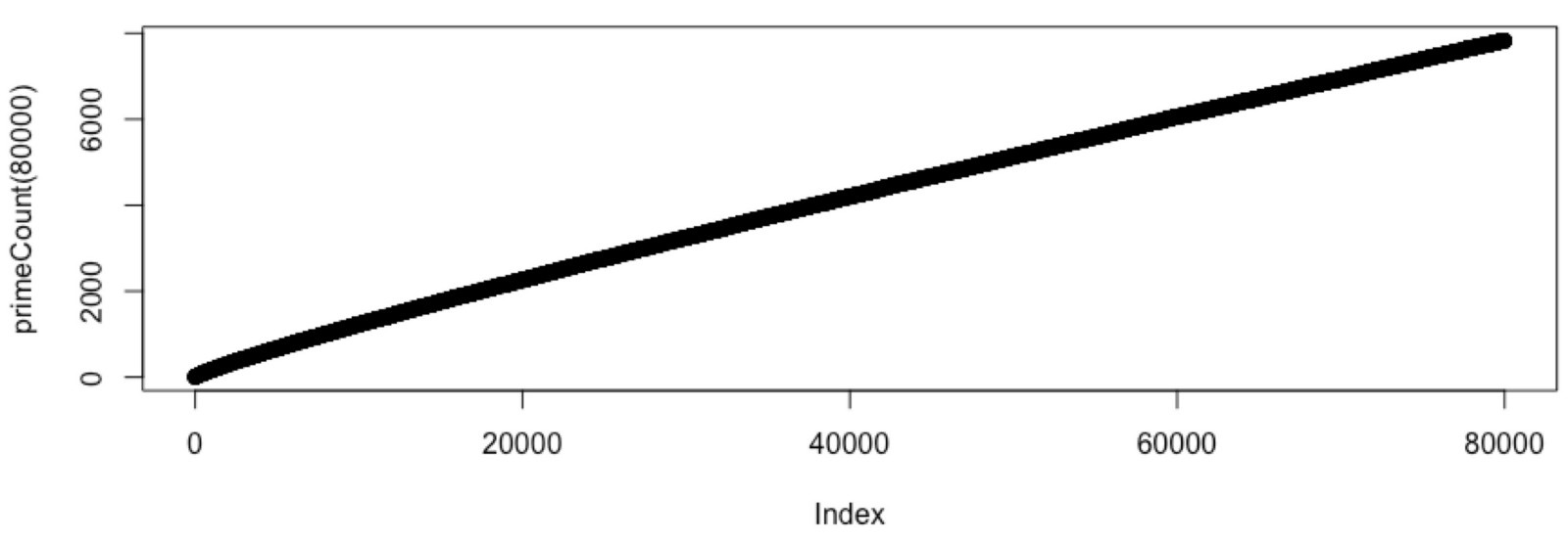
It may seem ridiculous that the prime numbers would eventually stop, but this idea is not such a radical one. If we count the prime numbers that we find up to a given point, we see that they become rarer and rarer as the integers become larger (see figure below). What is to say that we don’t eventually run out of prime numbers? (And why, if your teacher told you that the primes go on forever, did you believe them?)
The infinitude of the prime numbers
The proof that there are infinitely many prime numbers is another one of Euclid’s gems. This chapter has become long, but the proof is so beautiful that we must show it in case you have not seen it. (If you have seen this proof, then feel free to skip this section.)
Before proving that there are infinitely many primes, we state a mathematical fact that we will use soon.
Fact: Every composite integer larger than 1 has at least one prime factor.
Why is this fact true? Consider any composite integer n; because n is composite, it has factors other than itself and 1. Consider the smallest of these factors, which we call p. There is no way that p can be composite, since if it were, it would itself have a divisor other than itself and 1, which would also be a factor of n. This cannot be true since p is the smallest factor of n.
The above fact will prove useful when we replicate Euclid’s argument in the following theorem.
Theorem: There are infinitely many prime numbers.
To prove this theorem, we will employ an approach called proof by contradiction, in which we assume the opposite of what we want to demonstrate and show that it must be false. In this case, the opposite of what we want to prove is that there are finitely many prime numbers. How can we show that this statement is false?
Since we are assuming that there are finitely many primes, we can use the variable n to refer to the total number of these primes. Furthermore, we can label all of these primes using the notation p1 , p2 , . . . , pn . Consider the number q formed as the product of all the primes:
q = p1 · p2 · ⋯ · pn .
STOP: Is q composite? Why or why not?
Certainly, q is composite because all of the primes pi must be divisors of q. However, consider the number p that is one more than q:
p = q + 1 = (p1 · p2 · ⋯ · pn) + 1 .
STOP: Is p composite? Why or why not?
Because p is clearly larger than all of the finitely many primes pi, it must be composite. Yet consider what happens when we divide each prime into p. If we divide p1 into p, we obtain p2 · p3 · ⋯ · pn with a remainder of 1. If we divide p2 into p, we obtain p1 · p3 · p4 · ⋯ ·pn with a remainder of 1. And so on; any prime pi that we divide into p leaves a remainder of 1.
In short, none of the finitely many primes pi is a divisor of p. But according to the fact presented before this theorem, p must have some prime factor. It is impossible for these two statements to be true, and so we obtain a contradiction. Because our only assumption was that there are finitely many primes, we can conclude that the primes are infinite.
Factorials, arrays, and Eratosthenes’ insight
Now that we have proven that the primes really do march on forever, we return to Eratosthenes and his desire to find primes quickly. To help illustrate his insight, we will use a simpler example.
Say that you had gone to the effort of computing 100! by hand, and then someone asked you what 101! is. The last thing you would do would be to start multiply 1 by 2 by 3, and so on. Rather, you would simply multiply 100! by 101. What we are getting at is that it makes sense to store intermediate factorials that we obtain in a table rather than discarding them along the way.
In general, a table or ordered list of n variables is called an array of length n. If the name of our array is a, then the first variable in the array is denoted a[0], the second variable is denoted a[1], and so on. The numbers 0, 1, and so on are called the indices of the array. You have probably noticed that we use 0-based indexing of the array, in which we start counting indices at 0 instead of 1, a paradigm that may be alien but that is used by most modern programming languages.
STOP: What is the index of the last variable in an array of length n?
For the factorial example, we want a[0] to equal 0! = 1, a[1] to equal 1! = 1, a[2] to equal 2! = 2, a[3] to equal 3! = 6, and so on, up until a[n] = n!. Note that the length of this array is n + 1. We can state the generation of this array as a computational problem.
Factorial Array Problem
Input: An integer n.
Output: An array of length n + 1 containing the values 0!, 1!, 2!, . . . , n!
The following pseudocode solves the Factorial Array Problem, and it requires only a slight modification to the AnotherFactorial()
FactorialArray(n)
    a ← array of length n
    a[0] ← 1
    for every integer k between 1 and n
        a[k] ← a[k−1]·k
    return a
Exercise: The Fibonacci numbers are the classical sequence of integers given by (1, 1, 2, 3, 5, 8, 13, 21, …), in which the first two members of the sequence are equal to 1, and every subsequent number is equal to the sum of the two preceding numbers. Write a functionthat takes as input an integerFibonacciArray()nand returns an array containing the firstnFibonacci numbers.
We can now state our problem of finding primes as an array problem.
Prime Number Array Problem
Input: An integer n.
Output: An array primeBooleans of length n + 1 such that for every positive integer p ≤ n, primeBooleans[p] isif p is prime and primeBooleans[p] istrueotherwise.false
The following pseudocode implements the trivial algorithm for prime finding to solve the Prime Number Array Problem. Note that this function calls IsPrime()
TrivialPrimeFinder(n)
    primeBooleans ← array of n + 1 false boolean variables
    for every integer p from 2 to n
        if IsPrime(p) is true
            primeBooleans[p] ← true
    return primeBooleans
Much like our reasoning with FactorialArrayTrivialPrimeFinder
In this example, our largest number is n = 120. We start with p = 2 and cross off all multiples of 2, immediately concluding that almost half of the numbers considered are composite. We then look at the next number, p = 3, which is prime, and so we cross off all multiples of 3. Since p = 4 is composite, we skip it, as multiples of 4 will have already been labeled composite since they are also multiples of 2. In this manner, we cross off multiples of 5 and 7. Since 8, 9, and 10 are composite, we do not need to cross off their multiples. The next prime number would be 11, but note that 11 is larger than √120 = 10.954… The multiples of this number stop at 11 · 10 = 110, and therefore will already have been labeled composite in a previous step. We can therefore halt the process and look at all remaining numbers that have not been crossed off; these numbers (11, 13, 17, 19, etc.) must all be prime.
The following pseudocode implementing the Sieve of Eratosthenes starts by assuming that every number (other than 1) is prime. At each step, it looks for the smallest prime that we have not already identified, and then crosses off all multiples of this prime (for which it employs a subroutine called CrossOffMultiples).
SieveOfEratosthenes(n)
    primeBooleans ← array of n + 1 true boolean variables
    primeBooleans[0] ← false
    primeBooleans[1] ← false
    for every integer p between 2 and √n
        if primeBooleans[p] = true
            primeBooleans ← CrossOffMultiples(primeBooleans, p)
    return primeBooleans
As for the CrossOffMultiples() subroutine, it takes an existing array primeBooleans of Boolean variables as input along with an integer p. For every integer k that is a multiple of p between 2p and the final index of the array, this function sets primeBooleans[k] equal to false, which corresponds to “crossing off” these integers in the Sieve of Eratosthenes table. It then returns the updated primeBooleans array.
Note: A tricky part about theCrossOffMultiples()function is its first line. Recall that in 0-based indexing, the indices of an array having length k range from 0 to k – 1. As a result, in the pseudocode below, we set n equal to 1 less than the length ofprimeBooleans, which we access using alengthfunction that is typically built into programming languages for determining the length of an input array.
CrossOffMultiples(primeBooleans, p)
    n ← length(primeBooleans) - 1
    for every multiple k of p (from 2p to n)
        primeBooleans[k] ← false
    return primeBooleans
Exercise: It is possible to makeeven faster. If you are mathematically inclined, see if you can see how. (Hint: do we ever cross off integers that have already been crossed off?)SieveOfEratosthenes()
Forming a list of prime numbers
We now have two prime-finding algorithms. Yet if someone were to ask us what the prime numbers up to some positive integer n are, we would currently only be able to give them an array of boolean variables, where a variable is true if the number is prime and false otherwise. It would be better to provide a list of the integers that are prime.
The list of primes can be represented by an array primes. Although there are ways of estimating the number of primes up to and including n, we will not know how long this array should be in advance. Instead, we will start primes as having no elements; we will then append every prime number p found to the end of the array. After this process, primes will store the prime numbers between 2 and n in increasing order. The following pseudocode for a function ListPrimes()SieveOfEratosthenes()append
primes ← append(primes, p)
indicates that we take an array primes and an integer p as input, append p to primes, and then return this array, which we use to update primes.
ListPrimes(n)
    primes ← array of integers of length 0
    primeBooleans ← SieveOfEratosthenes(n)
    for every integer p from 0 to n
        if primeBooleans[p] = true
            primes ← append(primes, p)
    return primes
The sieve of Eratosthenes slaps
In the code-alongs accompanying this chapter, we will implement TrivialPrimeFinder()SieveOfEratosthenes(). The table below contains the run times of our implementation for a variety of different input values of n for these functions. Each row of this table also contains the speedup obtained from running SieveOfEratosthenes()TrivialPrimeFinder()
| n | | | Speedup |
| 10,000 | 0.0133 s | 0.000871 s | 15 |
| 100,000 | 0.226 s | 0.00990 s | 23 |
| 1,000,000 | 5.01 s | 0.104 s | 48 |
| 10,000,000 | 55.9 s | 0.930 s | 60 |
TrivialPrimeFinder()SieveOfEratosthenes()The table above exemplifies a general rule, which is that the larger an input dataset we provide to two algorithms, the greater the speedup for the faster algorithm. We hope that you now see why speed is such an important consideration when designing algorithms, especially in the modern era, as the amount of data that we are generating is growing at an ever-faster rate. As a result, we need fast algorithms more than ever before, and even a small efficiency improvement can mean a huge speedup at the scale of large data.
Even given the clear need for efficient algorithms, it may not seem as though prime numbers have any relevance to modern computing. And yet the ability to find large prime numbers quickly is central to a fundamental development in computer science called public key cryptography that we use every day, which we discuss in this chapter’s closing section.
Public key cryptography depends on finding primes
A fundamental property of the internet is that when you transmit a message (email, bank transaction, or even a private Google query), this message should be understood by the recipient, but not by anyone else who may be eavesdropping on the transmission. We therefore need to encrypt, or transform the message in some way, so that only the desired recipient can decrypt the transmission on the other end of the channel to reveal the original message.
Most encryption schemes that we might imagine are called symmetric, meaning that we use the same approach for encrypting and decrypting the message, called a key. For example, say that we encrypt a word by taking the next letter in the alphabet for each character, so that HELLO becomes encrypted as IFMMP. This key is symmetric because we can decrypt a message by taking the previous letter in the alphabet at each position. Although a code-breaker could quickly unravel this scheme, there is a much greater problem that arises for symmetric encryption approaches, which is that the key is private; the sender and receiver must agree upon the scheme in advance, since sending it on a public channel would defeat the purpose of encryption altogether. Private-key approaches are generally useless online, where we cannot meet the recipients of our messages in person. Private keys also present an apparent catch-22: the key itself is a message that we want to hide from eavesdroppers.
This straightforward problem of information-hiding seemed unsolvable for most of human history, until the late 1970s, when three mathematicians devised a new encryption scheme based on a public key. Their critical insight was that knowing the key used for encryption does not automatically imply that it is easy to decrypt the message, if the recipient knows certain additional details about the key.
This may sound mystical, but say that the recipient picks two very large prime numbers p and q (they may be around 300 digits long in practice), and form n = p · q, which they publish as the public key. Without getting into the details of how the encryption is performed, the key will be asymmetric in that knowing n does not help an eavesdropper know how to decrypt the encrypted message; the only way to decrypt the message is to know the primes p and q. No one has ever found an algorithm that can quickly factor a very large number n, and so someone listening in on the channel who sees the encrypted message will not be able to determine p and q; the recipient, on the other hand, knows these numbers and can decrypt the encrypted message quickly.
Public key cryptography exemplifies a seminal idea in computer science that rests on a foundation of beautiful mathematics. In the next chapter, we will see how computation can be used to find answers to biological questions without needing to run a single experiment, and we hope that you will join us. In the meantime …
It’s time to code!
We still have so much to do! You may still be skeptical that two algorithms for something as straightforward as finding prime numbers could really be different in terms of performance. So let’s learn some coding basics, and use them to implement these two algorithms and time them so that we can see for ourselves how fast the ancient Greeks’ algorithms for calculating a GCD and finding primes really are.


