Defining a tree
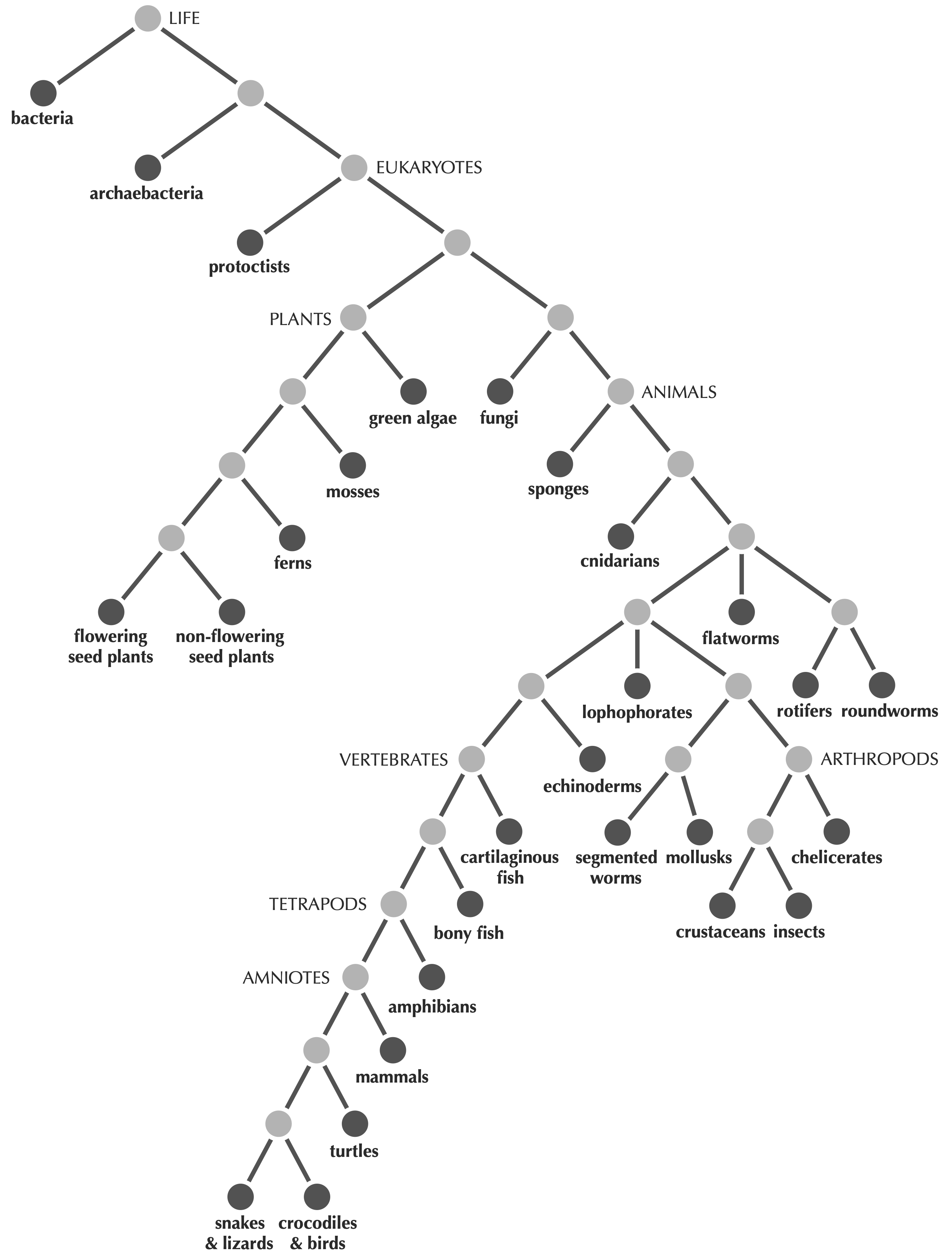
We begin with resolving the issue of what precisely we mean by a tree. Defining a tree precisely might not seem important, since we know that we want to build a tree of life like the one shown in the introduction or in the figure below.
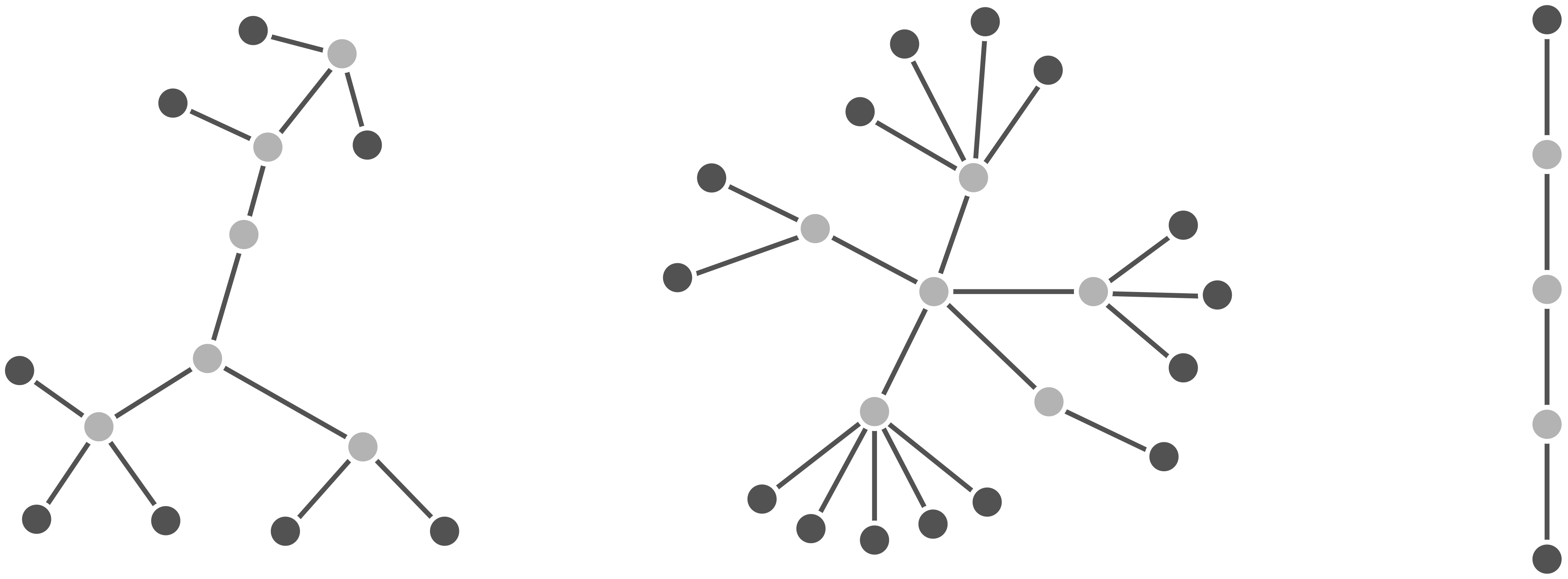
Fortunately, God gave the world mathematicians, who dictate that a tree is a connected, acyclic network. By connected, we mean that every pair of nodes in the network must be joined by some path (i.e., a sequence of edges); by acyclic, the network does not contain “cycles”, in which a path of edges leaves a node via one edge and returns via another. The figure below shows a collection of trees.
STOP: Why do you think these two properties (connected and acyclic) are important to the definition of a tree?
Let’s examine each of the two properties of a tree (connected and acyclic) to see why these properties are vital in order to provide a biological model of evolution. To this end, we will consider the consequences if each assumption does not hold.
First, if a tree were not connected, then we would obtain a network like that shown in the figure below, which can be divided out into “connected components”. Such a network is not biologically meaningful because it would imply that the organisms represented within the tree do not share a common ancestor. It may somehow be the case that there are groups of living things on Earth that do not share a common ancestor (moss piglets or the Finns could have extraterrestrial origins), but all of evolutionary biology stands upon the unprovable yet compelling dogma that life on Earth derives from a single organism, called the last universal common ancestor.
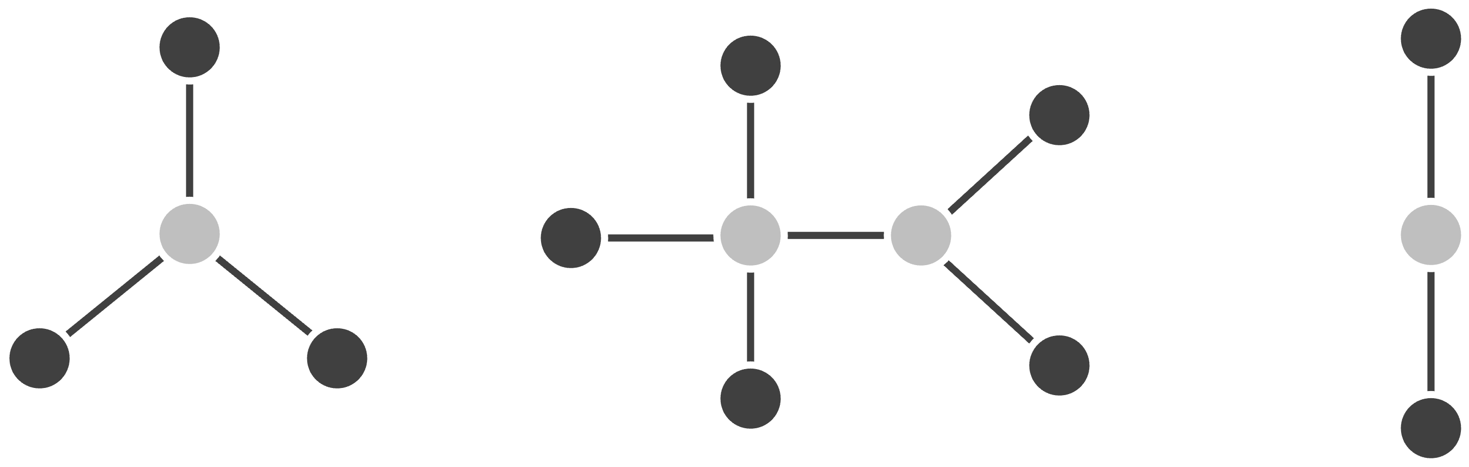
Second, students often think that a tree cannot have a cycle because a cycle would imply that evolution is traveling in two directions, but this assertion is not quite right. Consider, for example, the network shown in the figure below. This network has a cycle because two ancestral members combined genetic information to produce a new member of the network in an event called horizontal gene transfer.
Horizontal gene transfer might seem like a strange concept. Yet we observe an analogous phenomenon in the “family tree” of all humans, where recombination during sexual reproduction transfers genes between lineages. Horizontal gene transfer is also common in bacteria, which are the world’s largest commune and frequently exchange genes across species via mobile gene-carrying elements like plasmids. However, trees offer a great model for cross-species comparisons of eukaryotes (animals, plants, etc.). Furthermore, although horizontal gene transfer does occur in viruses, it is less common than in bacteria, making trees a great model for viral evolution.
A bit more about trees
You may have noticed that we colored some of the nodes in the trees above using darker gray. As Darwin indicated in this chapter’s epigraph, present-day species correspond to the outer “twigs” of the tree, whereas ancestral species are confined to interior nodes.
To make this idea more precise, we define the degree of a node as the number of edges incident to that node. Re-examining the tree from the start of this lesson (reproduced below), we see that the nodes of the tree divide into two types: leaves have degree equal to 1 and represent present-day species, whereas internal nodes have greater degree and represent ancestral species.
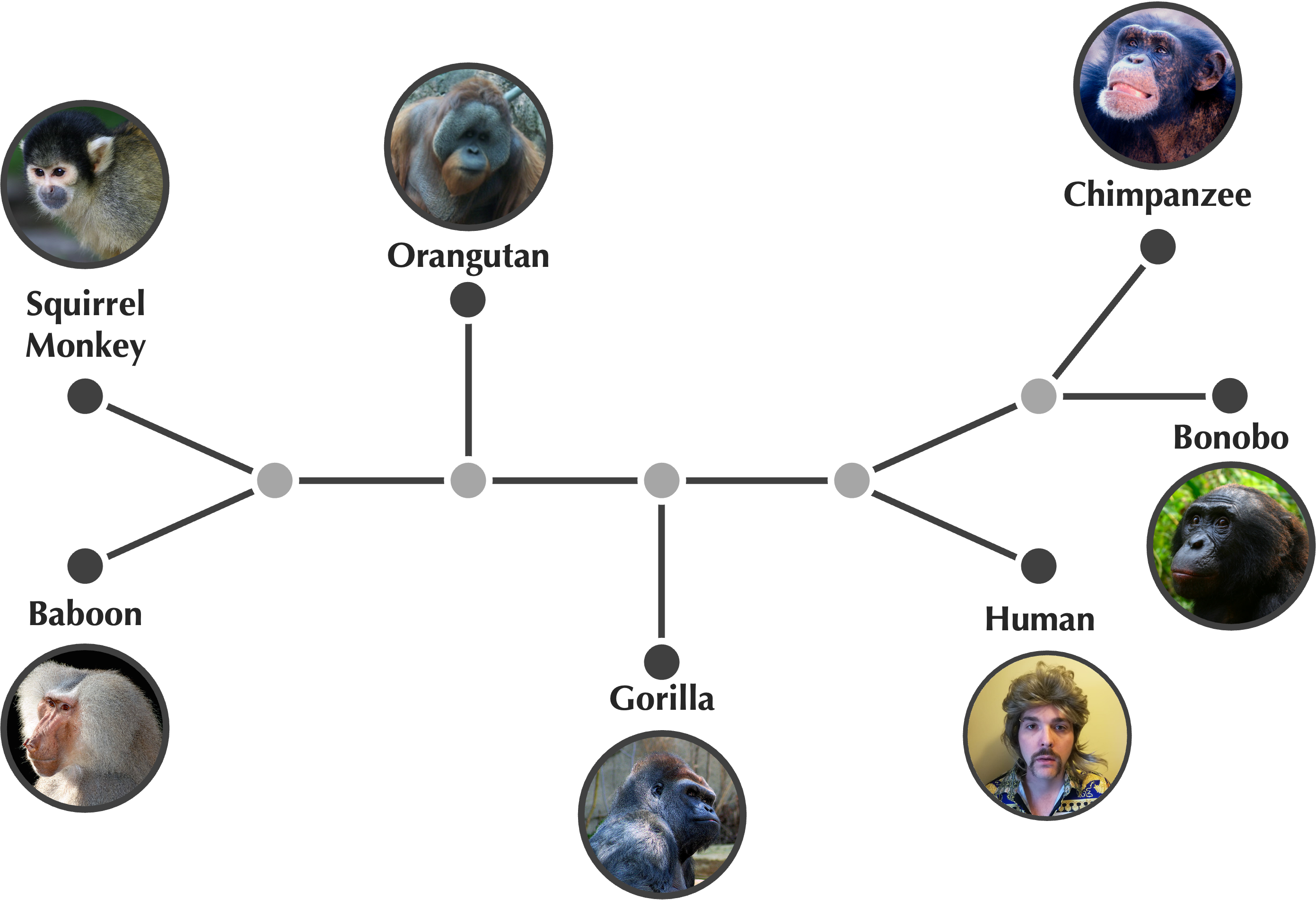
The node at the top of the tree above is called the tree’s root, since we infer it as the most recent common ancestor of all organisms represented in the tree. Often, inferring the root is a separate task to producing the tree. For example, consider the unrooted tree shown in the figure below. Students often assume that the most recent common ancestor of these beautiful organisms must exist somewhere in the middle of the tree, but the true root exists on the distant edge connecting the squirrel monkey to its most recent ancestor.
Now that we have a precisely defined notion of a tree, we return to our computational problem.
Distance-Based Tree Reconstruction Problem
Input: A distance matrix from a collection of species.
Output: An unrooted tree fitting the distance matrix.
Unfortunately, this problem is still not well defined because we need a notion of what it means for the tree to “fit” a distance matrix. The following exercise will allow you to explore how we might make this definition more concrete.
Exercise: Consider the distance matrix in the figure below, which we derived from a toy multiple alignment in the previous lesson. Find a tree that “fits” this distance matrix. (Hint: you should be assigning non-negative values to edges in a way that represents the information contained in the matrix.)
| Chimp | Human | Seal | Whale | |
| Chimp | 0 | 3 | 6 | 4 |
| Human | 3 | 0 | 7 | 2 |
| Seal | 6 | 7 | 0 | 2 |
| Whale | 4 | 5 | 2 | 0 |
Fitting a tree to a matrix
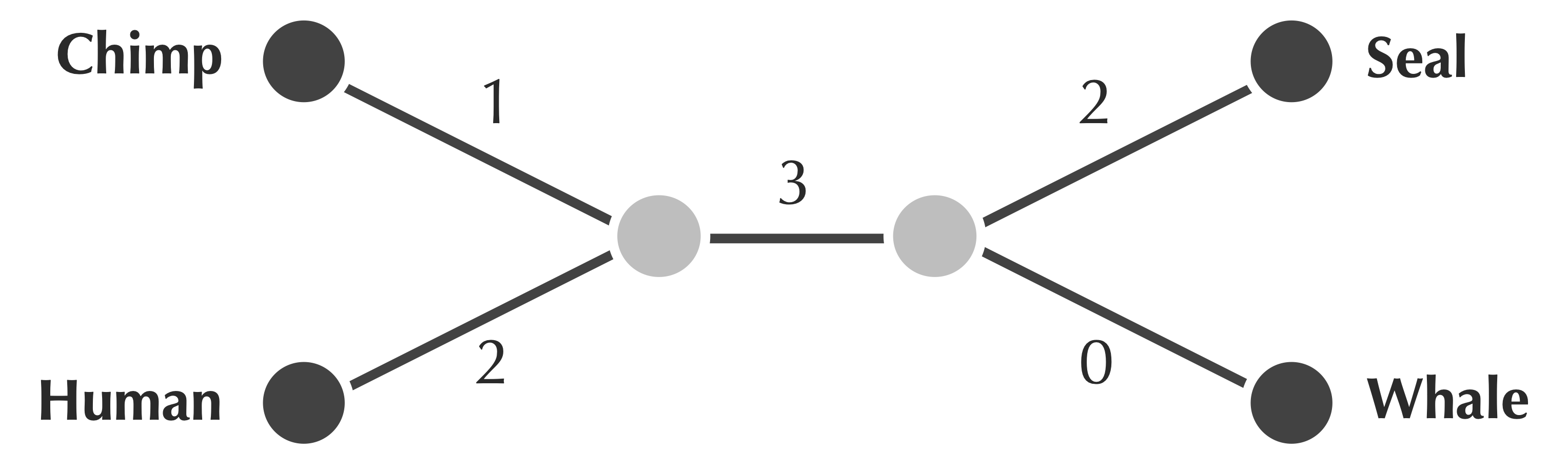
The figure below shows a tree fitting the matrix from the exercise at the end of the preceding section. We can nowrigorously establish that to fit a distance matrix, a tree must also have a collection of edge weights such that the sum of edge weights along the path connecting two leaves equals the value in the distance matrix corresponding to the distance between these species.
For example, the path from chimp to seal in the tree below accumulates edge weights of 1, 3, and 2, summing to 6, which equals the distance matrix value connecting chimp and seal. You may like to confirm that the paths connecting all other pairs match their distances in the matrix.
STOP: (For the mathematically inclined) Why do we know that there is only a single path connecting any two leaves in a tree?
Searching for an algorithm to fit a tree to a matrix
Now that we have a well-defined computational problem of finding an unrooted tree that fits a given distance matrix, we turn to designing an algorithm to solve it.
In solving our toy exercise, you may have noticed that the smallest element in the matrix (2), which connects seal to whale, corresponds to leaf nodes that are “adjacent” in the tree that fits the matrix. We could formalize this by saying that two leaves in a tree are neighbors if they share the node to which they are connected. Perhaps, then, the minimum value of the matrix corresponds to neighbors?
Sadly, this is not always true. Consider the matrix shown in the figure below.
| i | j | k | l | |
| i | 0 | 13 | 21 | 22 |
| j | 13 | 0 | 12 | 13 |
| k | 21 | 12 | 0 | 13 |
| l | 22 | 13 | 13 | 0 |
One might imagine that j and k should be neighbors in the tree fitting this matrix. Yet the tree that fits this matrix is shown in the figure below, in which j and k are connected by a path with three edges. As a result, inferring neighbors from the matrix’s smallest element provides a flawed starting point for our algorithm.
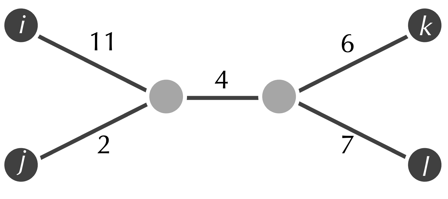
STOP: What property of the tree above makes j and k seem like neighbors when they are not? (Hint: consider the distances from each leaf node to its adjacent node.)
The astute reader may have noticed that we keep referring to “the tree” that fits a distance matrix. Why is this assumption valid? Perhaps there is another tree that also fits the data in the matrix above in which j and k are neighbors.
Indeed, more than one tree can fit the same data, as shown in the figure below, which shows a different tree fitting our first toy matrix with chimp, human, seal, and whale.
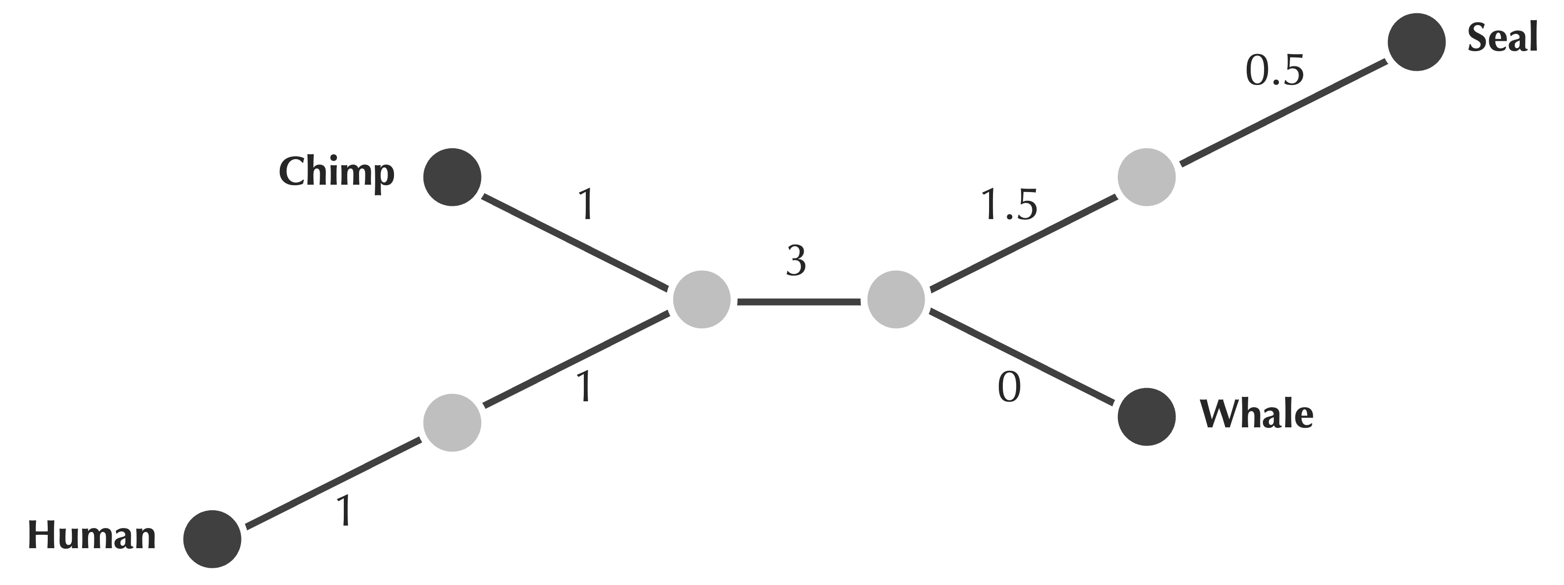
Of course, this tree is quite similar to the one that we showed previously, reproduced below, which you probably prefer because it does not contain any extraneous nodes. A fancier fancy way of saying this is that the tree below is simple, meaning that it contains no nodes having degree equal to 2.
It turns out that the mathematicians provide us with a concrete proof that any simple tree fitting a matrix is the unique simple tree fitting a matrix. We can therefore have confidence that the simple tree fitting a matrix is the best possible interpretation of the evolutionary history represented by that matrix.
Note: Although it lies beyond the scope of our work here, you can find a proof of this theorem, which was first established by Buneman in 1971, in my complementary Bioinformatics Algorithms project.
As it turns out, our problem is not that multiple trees might fit the same matrix. Our problem is that the overwhelming majority of distance matrices have no tree that fits them. For example, some dreaded linear algebra will demonstrate that the innocuous integer-valued matrix shown below has no tree that fits it.
| i | j | k | l | |
| i | 0 | 3 | 4 | 3 |
| j | 3 | 0 | 4 | 5 |
| k | 4 | 4 | 0 | 2 |
| l | 3 | 5 | 2 | 0 |
As a result, although we have placed evolutionary tree construction on a firm mathematical footing, we must abandon hope in a perfect evolutionary tree algorithm that produces the tree that fits a given distance matrix. Instead, the real evolutionary tree algorithms that have formed an area of research for decades are all heuristics, or approaches that find approximate solutions without guaranteeing a perfect result.
We will say more about heuristics in general in this course’s conclusion. In the meantime, we will transition to designing a heuristic that will construct an evolutionary tree for any distance matrix, even those that do not have a tree that fits them.