A first attempt at defining a computational problem for tree reconstruction
The scientific problem that we wish to solve has now come into focus.
Tree Reconstruction Problem
Input: A collection of species.
Output: A tree that best represents the evolutionary relationships among the species.
However, although this problem makes sense as a high-level scientific problem, a computer scientist looks at a problem like this with some puzzlement. What data do we have for each of the species in the input? Can we define a tree precisely? And what does it mean for this tree to “best represent” the relationships among the species?
The pitfalls of reconstructing trees from characters
Although these questions are all important, they were far from the mind of the 19th century biologists, who classified organisms using characters, or physical and anatomical characteristics that divide the organisms into groups.
For example, the predominant evolutionary division of dinosaurs is neither number of legs, nor dietary preferences, but rather hip bone shape. In 1888, Harry Seeley proposed this division after noticing that some dinosaur fossils had a pubis bone pointing downward and forward like modern reptiles, while others had a pubis pointing backward like modern birds. Seeley named the former group Saurischia (meaning “lizard-hipped”) and the latter group Ornithischia (meaning “bird-hipped), a division shown in the simplified figure below that has remained a cornerstone of paleontology for over a century.
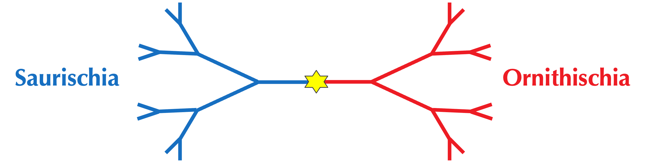
Note: Paradoxically, most paleontologists now believe that modern birds evolved from the lizard-hipped Saurischia, reiterating that age-old maxim that in biology, nothing makes sense.
STOP: Say that we are forming an evolutionary tree of all stick insects. What character might you use to divide the insects?
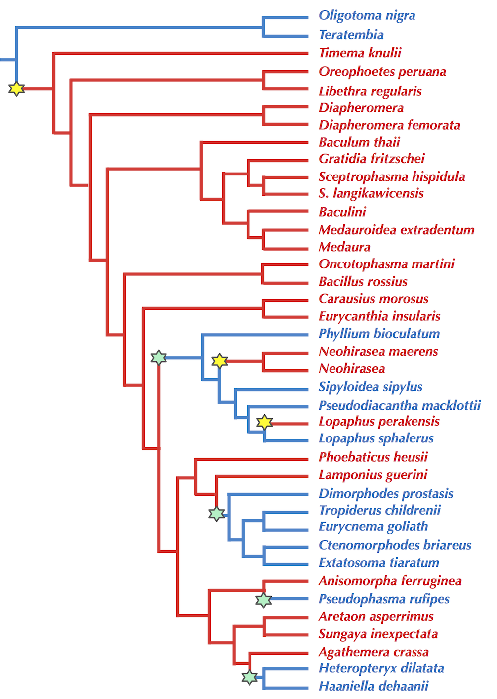
As students will reliably reply that Christopher Columbus (not Eratosthenes) discovered that the world is round, they will universally respond to the preceding question, “Wings!” And yet when we look at a published evolutionary tree of stick insects (figure below), our hypothesis that wings cleanly separate these species into two groups disintegrates.
Because using characters for tree reconstruction is flawed, we should transition toward an approach based on genetic data (i.e., DNA and proteins). This approach will prove much superior when it comes to analyzing viruses; after all, no microscope that has ever been manufactured would allow us to differentiate a coronavirus causing a pandemic from one that is harmless to humans.
Distance matrices provide a rich source of input data for tree construction
Fortunately, we live in an era in which genomic data, like those that we analyzed in Chapter 1, are plentiful. One common method for comparing n species is to form an n × n distance matrix D in which entry D[i, j] represents the distance between the i-th and j-th species. We should be comfortable with quantifying the distance between biological objects, since in Chapter 1’s practice exercises, we quantified the “beta diversity” between two metagenomic samples.
When building a distance matrix for a collection of species having known genomes, biologists often start with a multiple alignment of the same gene constructed from these species. Each row corresponds to a gene from one species, allowing us to analyze specific differences across the columns of the multiple alignment. The figure below shows a toy multiple alignment.
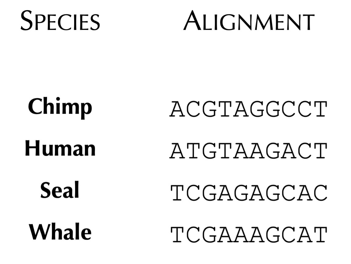
Note: If you are interested in studying algorithms for building multiple alignments of genes, then please check out our Bioinformatics Algorithms platform, where we devote two chapters to alignment algorithms.
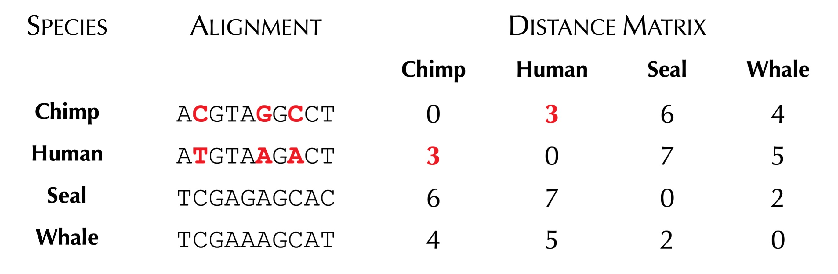
Once we are equipped with a multiple alignment, we can infer a distance matrix from it in a number of ways. One simple method is to count the number of differing symbols between corresponding columns. The distance matrix resulting from this computation for the toy multiple alignment above is shown in the figure below.
We now can reformulate our Tree Reconstruction Problem to include a distance matrix, as shown below.
Distance-Based Tree Reconstruction Problem
Input: A distance matrix from a collection of species.
Output: A tree corresponding to the distance matrix that represents the evolutionary relationships between the species.
We have now resolved the concerns about the input of this problem, but we must focus on the output as well. How can a tree “correspond” to a distance matrix? And what exactly is a tree, anyway?