Summing integers with lazy computer scientists
To introduce recursion, we consider the following computational problem, which we solved in the code alongs for Chapter 0. As you review this problem, take a deep breath and reflect on how far we have come.
Summing Integers Problem
Input: An integer n.
Output: The sum of the first n positive integers.
Imagine that we were intending to sum the first 100 positive integers by hand. We are not geniuses like Carl Friedrich Gauss, so we don’t know that the sum of the first n positive integers is equal to n · (n + 1) / 2; rather, we are budding computer scientists, for whom laziness and delegation is a virtue. Instead of summing all 100 numbers, we will delegate the task of summing the first 99 positive integers to a frenemy, and we will then add 100 to their result.
Sadly, the friend is also a computer scientist, and so they delegate the task of summing the first 98 positive integers to another computer scientist, with the intention of adding 99 to their result. The chain of delegation continues. At long last, the 99th computer scientist in the chain asks the 100th computer scientist to sum the first 1 positive integer. The 100th computer scientist, confused, replies, “1!”.
The 99th computer scientist then adds 2 to the result to obtain 3, which they communicate to the 98th computer scientist. The 98th computer scientist adds 3 to obtain 6, which they communicate to the 97th computer scientist. The 97th computer scientist adds 4 to obtain 10, which they communicate to the 96th computer scientist, and so on. Eventually, our frenemy (the 2nd computer scientist) adds 99 to 4,851 to tell us that the sum of the first 99 positive integers is 4,950.
Assuming that all these computer scientists’ arithmetic is correct, we now can add 100 to 4,950 to obtain that the sum of the first 100 positive integers is 5,050.
Recurrence relations imply recursive algorithms
More formally, if we denote the sum of the first n positive integers as S(n), then it is not exactly Earth-shattering to assert that
S(n) = n + (n – 1) + (n – 2) + … + 2 + 1 .
However, note that the final n – 1 terms of this summation correspond to S(n – 1). As a result, we can write the formula as
S(n) = n + S(n – 1) .
The above formula is called a recurrence relation because it establishes an equation involving a function f(x) in which f(x) can be expressed as equal to some combination of inputs f(y), where y is smaller or simpler than x.
Once we have established a recurrence relation, we can infer a recursive algorithm for computing the desired function. Our recursive algorithm for solving the Summing Integers Problem is called RecursiveSum() and is shown below.
RecursiveSum(n)
    if n > 1
        return n + RecursiveSum(n-1)
    else
        return 1
Every recursive algorithm consists of two components. First, the base case is a simple case in which the function usually returns a simple value, which in this case occurs when n is equal to 1 and the function returns 1. Second, the inductive step applies the recurrence relation to call the algorithm on a simple input, which in this case occurs when n is greater than 1 and the algorithm return n + RecursiveSum(n-1).
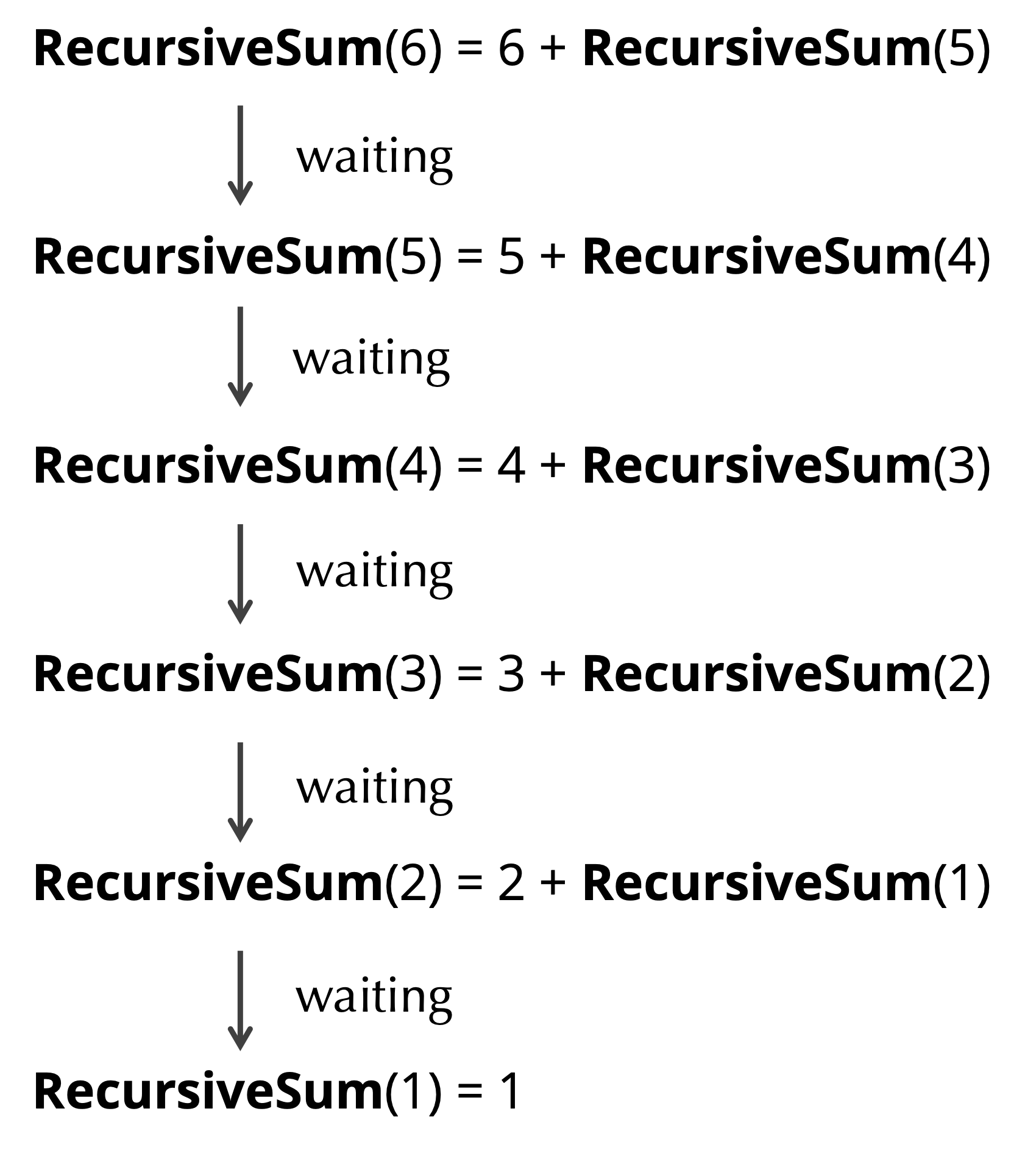
RecursiveSum() solves the problem of summing integers in the same way as the lazy computer scientists. For example, say that we call RecursiveSum(6). Because 6 is greater than 1, we consult the inductive step, which returns 6 + RecursiveSum(5). In other words, the algorithm delegates most of the work to a minion, the function call RecursiveSum(5). In turn, RecursiveSum(5) will return 5 + RecursiveSum(4), which means that it needs to wait for the minion RecursiveSum(4) to finish.
The chain continues, as shown in the figure below. In the process, all the RecursiveSum() calls that are waiting accumulate in the computer’s memory in a location called the function stack.
RecursiveSum(6).When RecursiveSum(2) calls RecursiveSum(1), the latter hits a base case since the input is equal to 1. As a result, this function returns 1, and RecursiveSum(2) can return 2 + RecursiveSum(1) , which is equal to 3. In turn, RecursiveSum(3) can now return 3 + RecursiveSum(2), which is equal to 6. Eventually, RecursiveSum(5) returns a value of 15, and RecursiveSum(6) can return our desired value of 15 + 6 = 21 (see figure below).
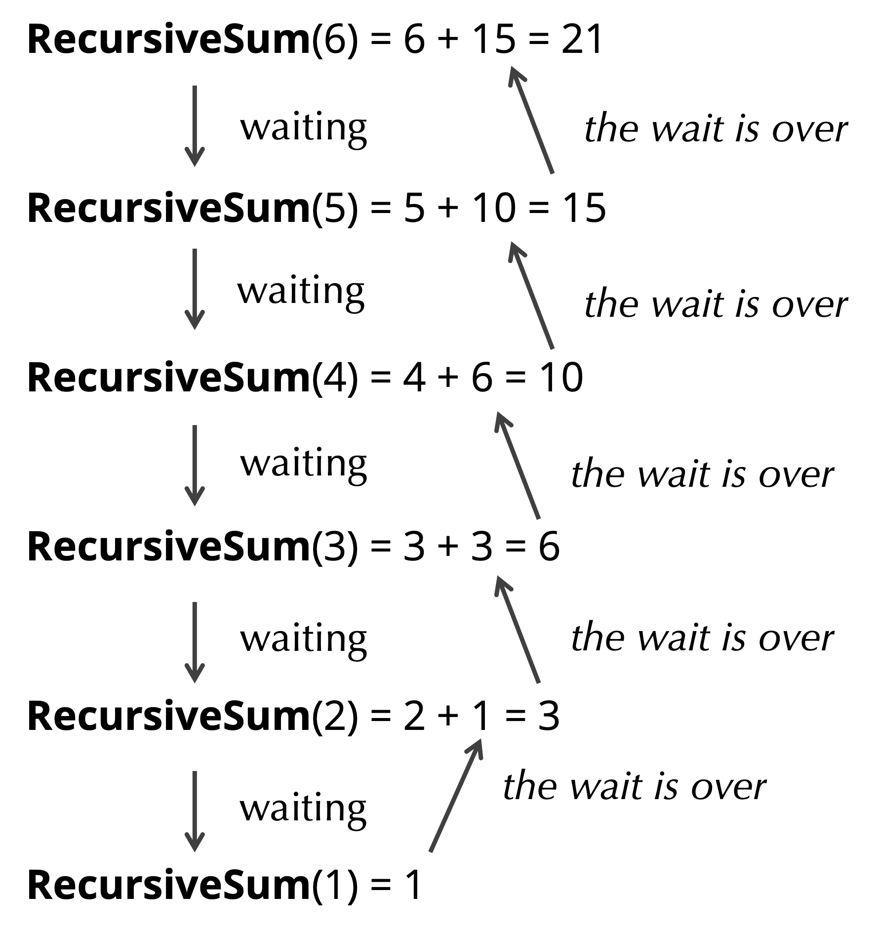
RecursiveSum(1) returns 1, it returns a value to RecursiveSum(2), which returns a value to RecursiveSum(3), and so on, until RecursiveSum(6) returns.STOP: Say that we forgot to provide a base case forRecursiveSum(), as shown in the following pseudocode. What would happen if we calledRecursiveSum(6)? (Hint: eventually,RecursiveSum(1)will be called; what happens?)
RecursiveSum(n)
    if n > 1
        return n + RecursiveSum(n-1)
Two exercises on recursion: factorial and Fibonacci
Before we return to counting leaves in trees and UPGMA, we will consider two exercises to allow us to practice what we have learned. In each case, first establish a recurrence relation, and then use this recurrence relation to design a recursive algorithm.
Exercise: Write pseudocode for a recursive functionRecursiveFactorial()that takes as input an integernand returns the factorial ofn.
The solution to this exercise is shown below.
RecursiveFactorial(n)
    if n > 0
        return RecursiveFactorial(n – 1) * n
    else
        return 1
Note: The order in which inductive steps and base cases are presented typically does not matter. For example, the following pseudocode forRecursiveFactorial(), in which the order of the base case and inductive steps have switched in the if statement, will also return the factorial ofn.
RecursiveFactorial(n)
    if n = 0
        return 1
    else
        return RecursiveFactorial(n – 1) * n
Exercise: Write pseudocode for a recursive functionRecursiveFibonacci()that takes as input an integer n and returns the n-th Fibonacci number, using 0-based indexing. That is,RecursiveFibonacci(0)andRecursiveFibonacci(1)should be 1,RecursiveFibonacci(2)should be 2,RecursiveFibonacci(3)should be 3,RecursiveFibonacci(4)should be 5, etc.
The problem with recursive Fibonacci
If Fib(n) denotes the n-th Fibonacci number, then the fact that the n-th Fibonacci number is formed as the sum of the previous two Fibonacci numbers provides us with a recurrence relation for Fib(n), which involves two calls to Fib().
Fib(n) = Fib(n-1) + Fib(n-2) .
We can use this recurrence relation to design a recursive algorithm called RecursiveFibonacci()solving the exercise from the previous section, as shown below. Note that the base case applies when n is equal to either 0 or 1, since the recurrence relation involves two terms.
RecursiveFibonacci(n)
    if n < 2
        return 1
    else
        return RecursiveFibonacci(n-1) + RecursiveFibonacci(n-2)
Let’s implement this algorithm in Python to see it in action. In the sandbox below, we print the first few Fibonacci numbers.
Let’s also see what happens when we call recursive_fibonacci(50).
Although we successfully called recursive_fibonacci() on smaller inputs, the call to recursive_fibonacci(50) times out! To understand what is happening, consider that when RecursiveFibonacci(n) is called, it in turn adds RecursiveFibonacci(n-1) and RecursiveFibonacci(n-2) to the function stack. That may seem innocuous, but consider the figure below, which shows the stack of all function calls generated by RecursiveFibonacci(7).
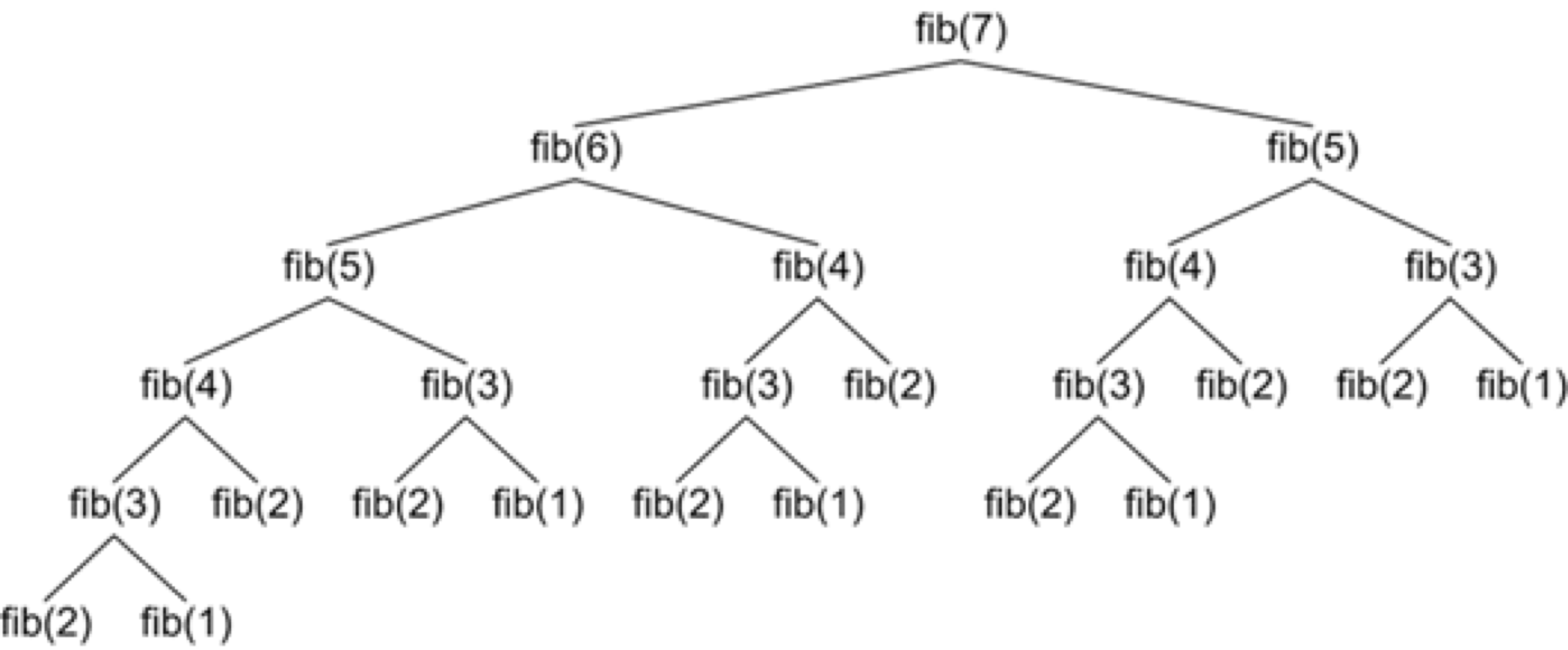
RecursiveFibonacci(7) (abbreviated here as fib(7)) is called. Courtesy: introprogramming.info.The problem, which did not occur in the case of computing sums or factorials recursively, is that many of the function calls shown in the figure above are repeated. For example, consider that RecursiveFibonacci(3) is called five times, with these function calls occurring independently.
Furthermore, because each function call accumulates two additional function calls onto the stack, the number of function calls on the stack grows exponentially as a function of n (it grows like 2n). As a result, when we call RecursiveFibonacci(n) for even modest values of n, we exhaust the memory allocated to the stack and produce stack overflow, crashing the program. This entire situation was summarized by a former student in just three memorable words: “big tree bad”.
The moral of recursion is that it offers an excellent approach for concisely representing solutions to problems in some cases, but we should be wary of recursive functions that rely on calling themselves multiple times, but only if it produces redundant independent function calls on the stack.
Exercise: We will next write a functionCountLeaves()that counts the number of leaves in the tree “rooted” at an input node. What is the recurrence relation? What are the base case and inductive step?
Counting leaves recursively
Fortunately, counting leaves recursively will not encounter the same issues as computing Fibonacci numbers. Given a node v, if the node is an internal node with child nodes u and w, then CountLeaves(v) is equal to the sum of the number of leaves in the subtrees whose roots are u and w. That is,
CountLeaves(v) = CountLeaves(u) + CountLeaves(w) .
This recurrence relation forms our inductive step. As for a base case, if v is a leaf, then CountLeaves(v) is equal to 1. We now can write our CountLeaves() subroutine, which is only three lines long. The pseudocode is so short that you might be skeptical that it works; if so, you will just have to join us for this chapter’s code alongs.
CountLeaves(v)
    if v.child1 = nil and v.child2 = nil
        return 1
    return CountLeaves(v.child1)  + CountLeaves(v.child2)
STOP: Why doesCountLeaves()not encounter the problems thatRecursiveFibonacci()did? (Hint: how large can the function stack be?)
Note: Technically, we might wish to ensure that our function can handle the case that a node has only one child instead of two. In this case, we need additional inductive steps that only return the number of leaves in the tree rooted at this solitary child, as shown below.
CountLeaves(v)
    if v.child1 = nil and v.child2 = nil
        return 1
    else if v.child1 = nil
        return CountLeaves(v.child2)
    else if v.child2 = nil
        return CountLeaves(v.child1)
    return CountLeaves(v.child1)  + CountLeaves(v.child2)
It’s time to code
UPGMA is now finished, and feel free to take another deep breath. You are now ready to learn even more about object-oriented programming in this chapter’s code alongs, where we will implement UPGMA and use it to visualize evolutionary trees of coronaviruses in order to see the rise and spread of SARS-CoV-2 variants. We hope you will join us!