Implementing UPGMA with Object-Oriented Programming

Two object-oriented designs for evolutionary trees

To design pseudocode representing the UPGMA algorithm, we should first establish our object-oriented design. To do so, we reproduce a tree produced by UPGMA below; we would like to represent the information in this tree in keeping with the principles of abstraction.

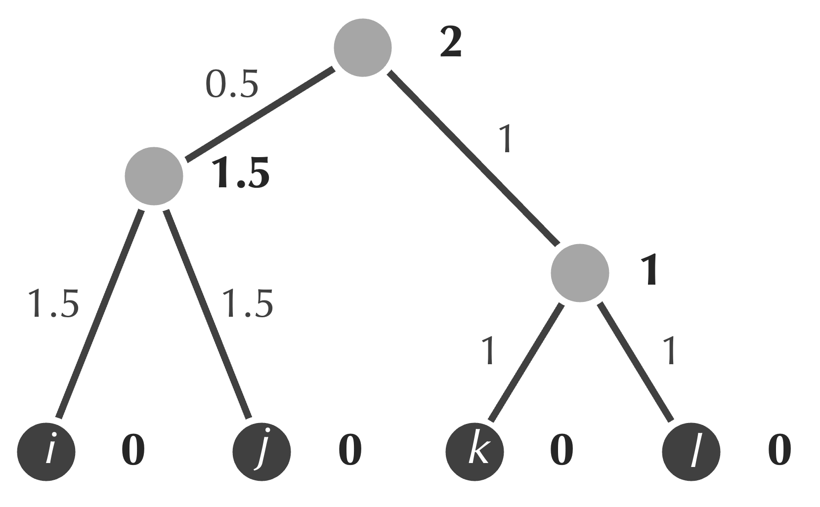
For example, recall that storing the area or perimeter of a Rectangle object in addition to its width and height would be redundant and lead to conflicting fields. Adapting the same mindset to evolutionary trees means that it would be redundant to store both the ages of nodes and the weights of edges, since we can always infer the weight of an edge by taking the positive difference of the ages of nodes that the edge connects.

Designing our data top-down, we might think of a Tree object as constituting a collection of Node objects and a collection of Edge objects, which we show below.

type Tree
    nodes []Node
    edges []Edge

type Node
    age float
    label string

type Edge
    parent Node
    child Node

In turn, each Node object should store its age and a label (e.g., corresponding to that node’s species name), and each Edge object should store two Node objects representing the nodes that it connects, which we call parent and child to preserve the edge’s orientation from the root toward the leaves.

type Tree
    nodes []Node
    edges []Edge

This design is a reasonable one, but we can implement UPGMA without needing to store the edges of the tree explicitly, since each Node object can simply store its two “children”. We will therefore adopt the following object-oriented design in implementing UPGMA, although we will see in the code alongs that this approach can be fraught with peril and will require us to have an appreciation of how a programming language manages memory.

type Tree
    nodes []Node

type Node
    age float
    label string
    child1 Node
    child2 Node

Walking through UPGMA: initializing the tree

When we walked through the steps of UPGMA on a toy dataset in the previous lesson, we specified these steps in human language. To convert these ideas to pseudocode, we need to think about how our objects will update at each step.

First, because we reduce the number of rows of the distance matrix by 1 in each step of UPGMA, we know that if we start with n rows of our distance matrix, then we will have n . For example, in the UPGMA tree above, we have four leaves and three internal nodes.

Therefore, the first thing that we will do is to initialize the tree t to have 2*numLeaves-1 total nodes, where numLeaves is equal to the number of rows in the input distance matrix D. We will pass this work to a subroutine InitializeTree(), as shown in our initial scaffolding of a UPGMA() function below. Note that UPGMA() takes as input both D and a collection of strings speciesNames, which we will use to assign label fields for the leaves of the tree in InitializeTree().

UPGMA(D, speciesNames)
    numLeaves ← CountRows(D)
    t ← InitializeTree(speciesNames)

    ...

    return t

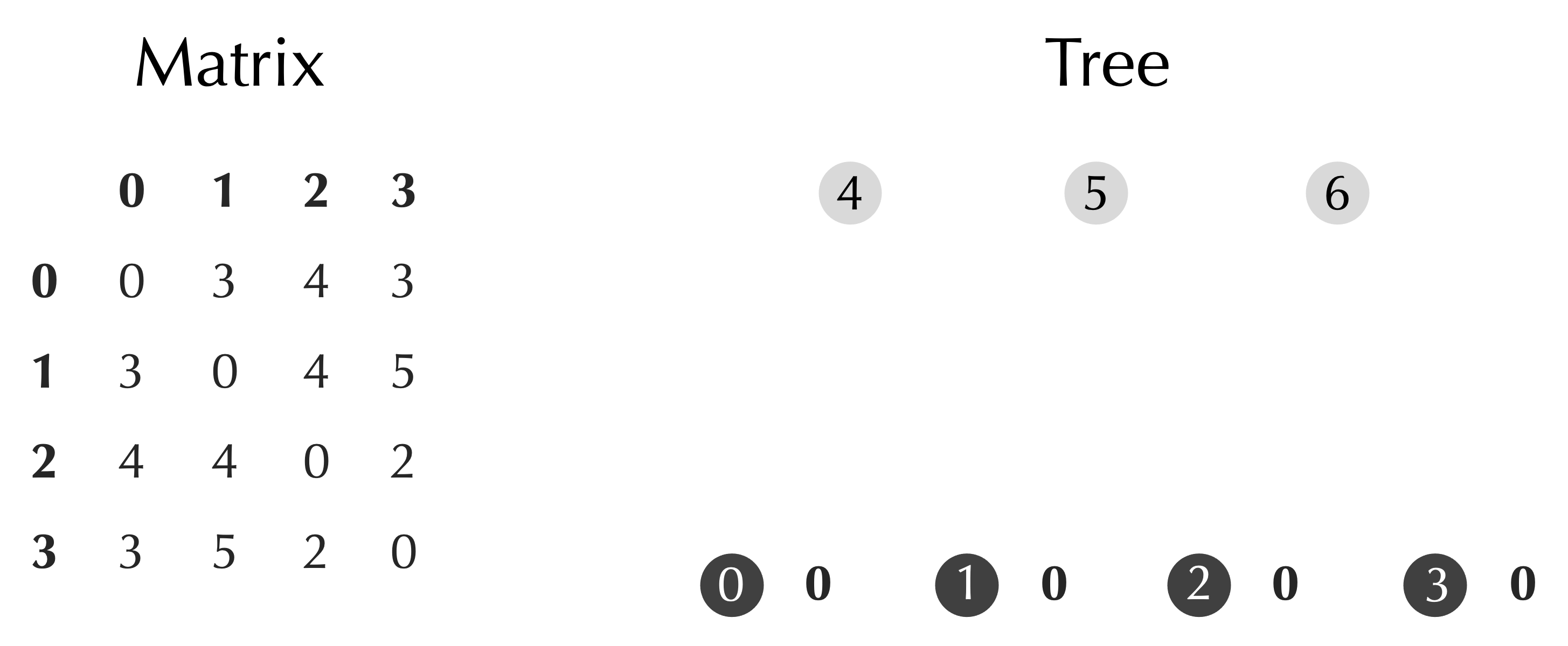
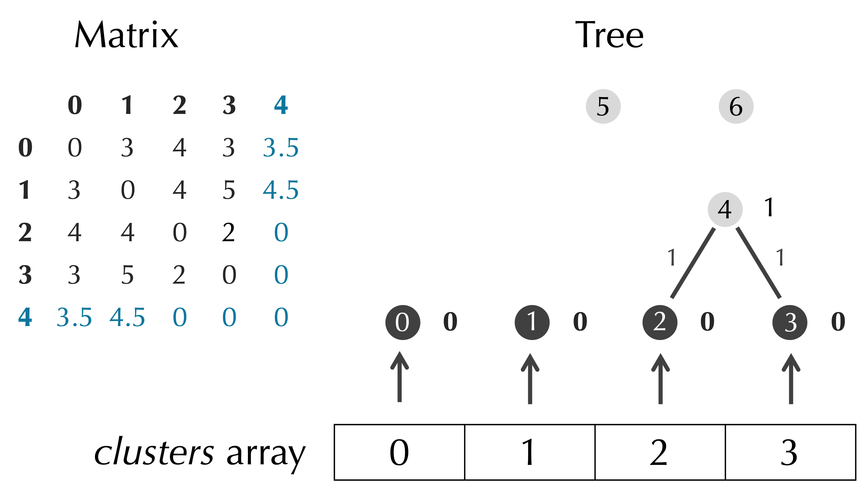
Let’s show how this works for our toy distance matrix from the previous section. After applying InitializeTree(), our data have the form shown in the figure below. Note that for simplicity, since there are no species names relevant to this toy dataset, we are providing the nodes with the names "0", "1", "2", etc. We also assign an age of zero to each leaf node.

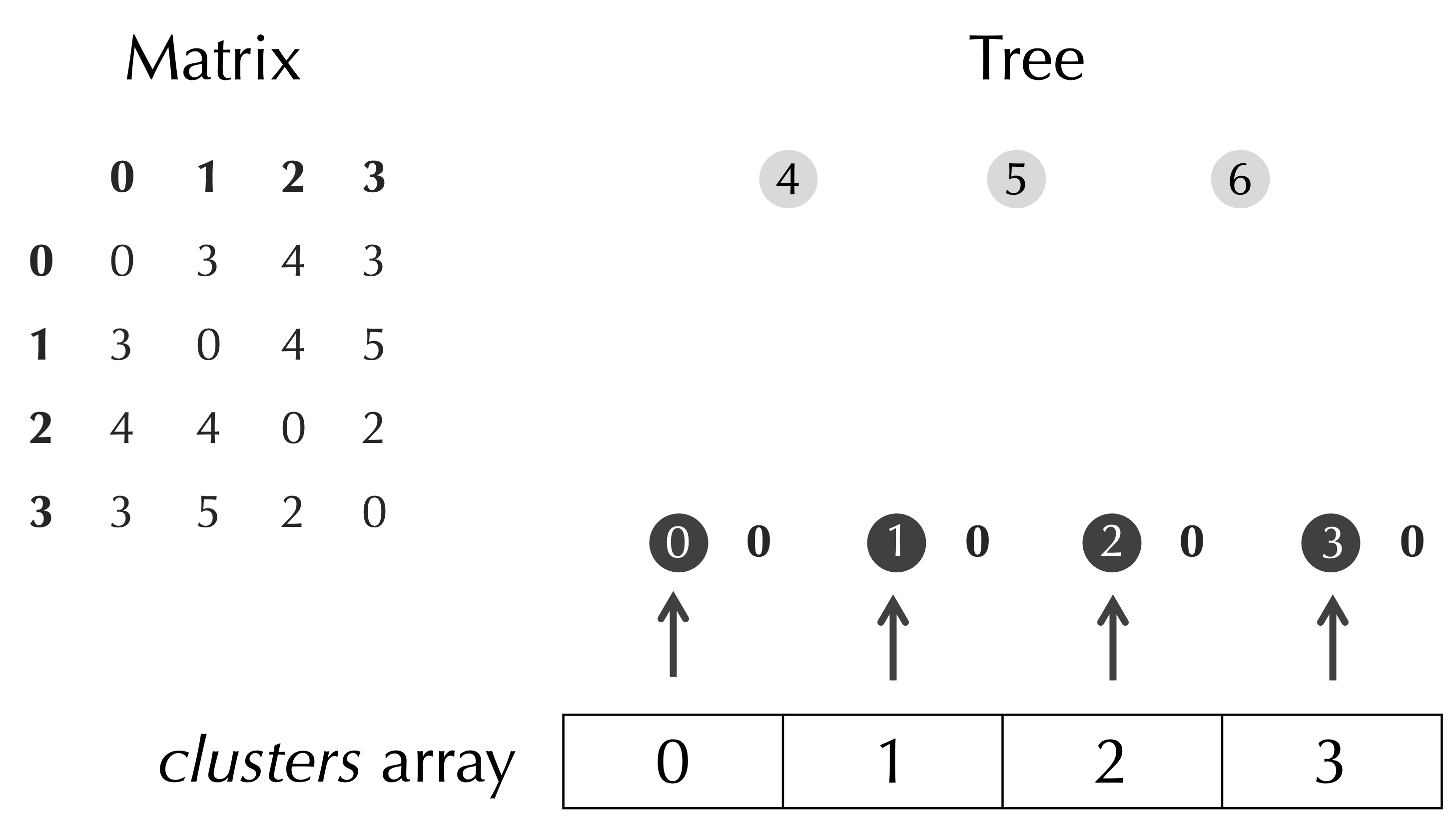
Next, we point out that as the matrix updates, we need to remember what each row and column correspond to. For example, in the first step of UPGMA, we will be merging nodes 2 and 3 together to form a new node, which will correspond to the third row of the matrix. We therefore will introduce an additional array clusters of Node objects such that clusters[i] refers to the Node represented in row i of the current matrix. At the start of the algorithm, clusters will refer to the leaf nodes of the tree, as shown below.

We can now add one line to UPGMA(), which calls InitializeClusters() to initialize the array clusters.

UPGMA(D, speciesNames)
    numLeaves ← CountRows(D)
    t ← InitializeTree(speciesNames)
    clusters ← InitializeClusters(t)

    ...

    return t

Walking through UPGMA: a single step of the algorithm

The engine of UPGMA will take numLeaves-1 steps, adding one node to the tree in each step. In particular, because we have already set the elements of t.nodes having indices between 0 and numLeaves-1, we will be setting t.nodes[p], where p ranges from numLeaves to 2*numLeaves - 2.

UPGMA(D, speciesNames)
    numLeaves ← CountRows(D)
    t ← InitializeTree(speciesNames)
    clusters ← InitializeClusters(t)
    for every integer p from numLeaves to 2*numLeaves–2

        ...

    return t

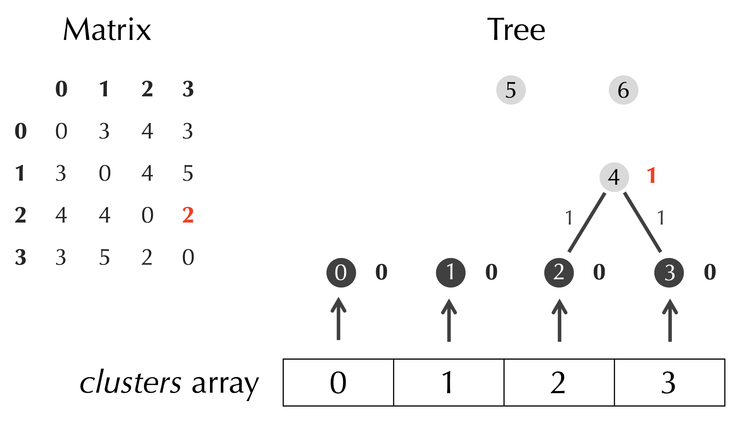
As with our walkthrough of UPGMA in the previous lesson, we will first find the minimum element of the matrix. To do so, we will write a subroutine FindMinElement() that takes as input a distance matrix D and returns a triplet: the row and column index (row and col) of the minimum value of D, followed by that minimum value (val).

Once we have determined the minimum value of D, we set the age of the current node, t.nodes[p], equal to half this value. This process is illustrated in the figure below.

Below, we continue to update our UPGMA() pseudocode.

UPGMA(D, speciesNames)
    numLeaves ← CountRows(D)
    t ← InitializeTree(speciesNames)
    clusters ← InitializeClusters(t)
    for every integer p from numLeaves to 2*numLeaves–2
        row, col, val ← FindMinElement(D)
        t.nodes[p].age ← val/2

        ...

    return t

As the figure above illustrates, we also need to connect t.nodes[p] to its two children. We are tempted to say that these two children are given by t.nodes[row] and t.nodes[col], which is correct for the example above. However, we will not always be connecting t.nodes[p] to two leaves; sometimes, we will be connecting it to internal nodes. For this reason, we maintain an array clusters that stores the current Node objects that are represented by the distance matrix, and we connect t.nodes[p] to the nodes corresponding to clusters[row] and clusters[col]. Note in the above example that clusters[row] and clusters[col] also point to t.nodes[2] and t.nodes[3].

UPGMA(D, speciesNames)
    numLeaves ← CountRows(D)
    t ← InitializeTree(speciesNames)
    clusters ← InitializeClusters(t)
    for every integer p from numLeaves to 2*numLeaves–2
        row, col, val ← FindMinElement(D)
        t.nodes[p].age ← val/2
        t.nodes[p].child1 ← clusters[row]
        t.nodes[p].child2 ← clusters[col]

        ...

    return t

We next update the distance matrix. We know that we will eventually transform our numLeaves × numLeaves matrix into a (numLeaves - 1) × (numLeaves - 1) matrix. However, we start by adding a row and column to the matrix to make it into a (numLeaves + 1) × (numLeaves + 1) matrix, where the final row and column corresponds to t.nodes[p] and formed from merging the two clusters corresponding to the minimum value of D, as shown in the figure below.

We pass the work of adding a row and column to D to a subroutine AddRowCol(), which will need to perform a weighted average based on the number of elements in the clusters that we are merging. Accordingly, we need to pass these cluster sizes as inputs into AddRowCol(). These cluster sizes are equal to the number of leaves in the trees whose roots are the two children of t.nodes[p]. We can now continue to update our pseudocode.

UPGMA(D, speciesNames)
    numLeaves ← CountRows(D)
    t ← InitializeTree(speciesNames)
    clusters ← InitializeClusters(t)
    for every integer p from numLeaves to 2*numLeaves–2
        row, col, val ← FindMinElement(D)
        t.nodes[p].age ← val/2
        t.nodes[p].child1 ← clusters[row]
        t.nodes[p].child2 ← clusters[col]
        clusterSize1 ← CountLeaves(t.nodes[p].child1)
        clusterSize2 ← CountLeaves(t.nodes[p].child2)
        D ← AddRowCol(D, clusterSize1, clusterSize2, row, col)

        ...

    return t

We have now merged together the clusters corresponding to the indices row and col, and we can delete the row and column of D at these indices, as illustrated below.

We pass the work of this deletion to a subroutine, and we update our pseudocode for UPGMA() accordingly.

UPGMA(D, speciesNames)
    numLeaves ← CountRows(D)
    t ← InitializeTree(speciesNames)
    clusters ← InitializeClusters(t)
    for every integer p from numLeaves to 2*numLeaves–2
        row, col, val ← FindMinElement(D)
        t.nodes[p].age ← val/2
        t.nodes[p].child1 ← clusters[row]
        t.nodes[p].child2 ← clusters[col]
        clusterSize1 ← CountLeaves(t.nodes[p].child1)
        clusterSize2 ← CountLeaves(t.nodes[p].child2)
        D ← AddRowCol(D, clusterSize1, clusterSize2, row, col)
        D ← DelRowCol(D, row, col)

        ...

    return t

As we updated the matrix, we will update the clusters array as well. We begin by appending a Node to clusters, which refers to our new node t.nodes[p], as shown below.

Because we have three rows in our matrix, we should have three elements in clusters, and so we can delete the Node objects in clusters corresponding to the rows and columns of D that we deleted, which are clusters[row] and clusters[col] (see figure below).

We pass the work of adding and deleting clusters to subroutines, as shown below in our UPGMA() pseudocode, which is now complete.

UPGMA(D, speciesNames)
    numLeaves ← CountRows(D)
    t ← InitializeTree(speciesNames)
    clusters ← InitializeClusters(t)
    for every integer p from numLeaves to 2*numLeaves–2
        row, col, val ← FindMinElement(D)
        t.nodes[p].age ← val/2
        t.nodes[p].child1 ← clusters[row]
        t.nodes[p].child2 ← clusters[col]
        clusterSize1 ← CountLeaves(t.nodes[p].child1)
        clusterSize2 ← CountLeaves(t.nodes[p].child2)
        D ← AddRowCol(D, clusterSize1, clusterSize2, row, col)
        D ← DelRowCol(D, row, col)
        clusters ← append(clusters, t.nodes[p])
        clusters ← DelClusters(clusters, row, col)
    return t

Walking through UPGMA: iterating over multiple steps

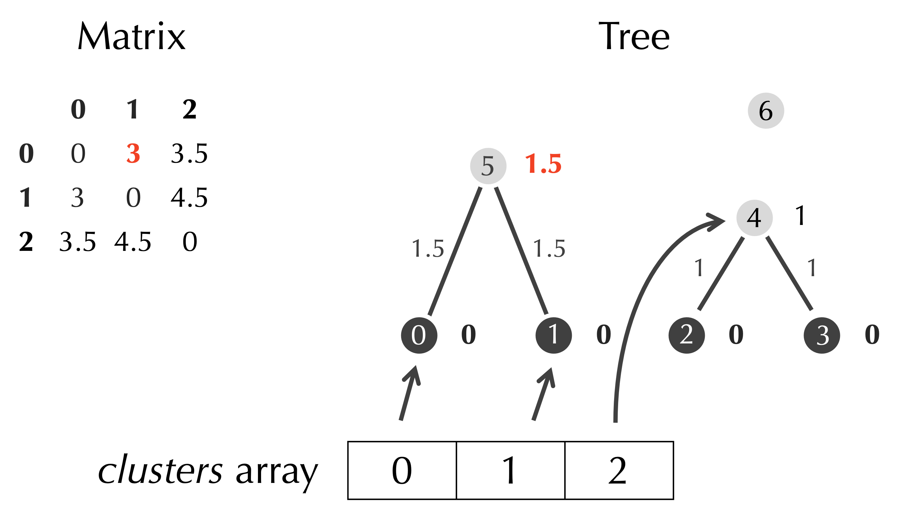
Although we have finished the pseudocode for UPGMA, we will use this section to illustrate how data update in subsequent steps of the algorithm, starting with adding the node with index 5.

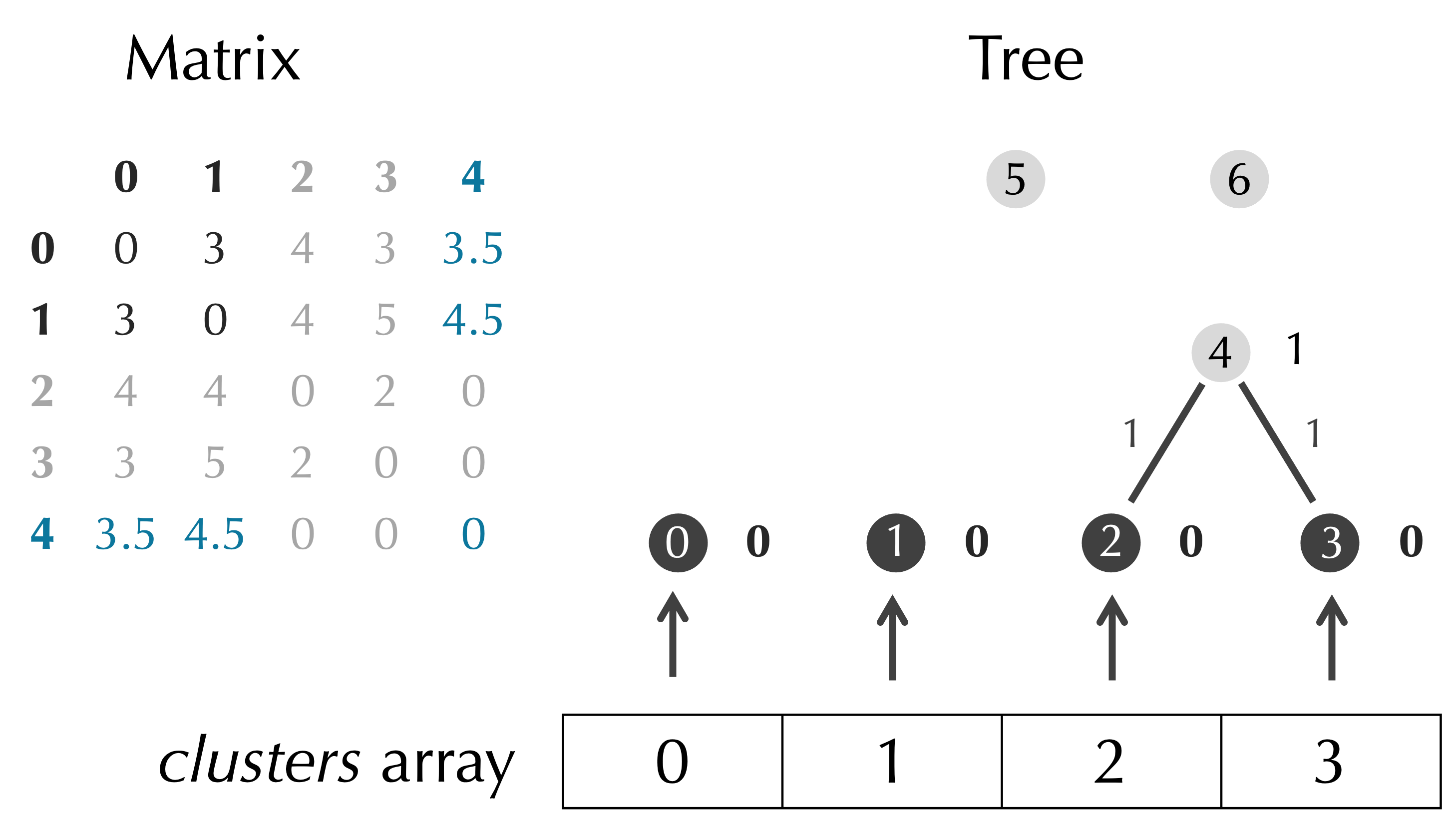
First, we identify the minimum element of the matrix of 3, which occurs when row is 0 and col is 1. We assign half the minimum value, 1.5, as the age of the new node, and connect this node to clusters[row] and clusters[col] via two edges.

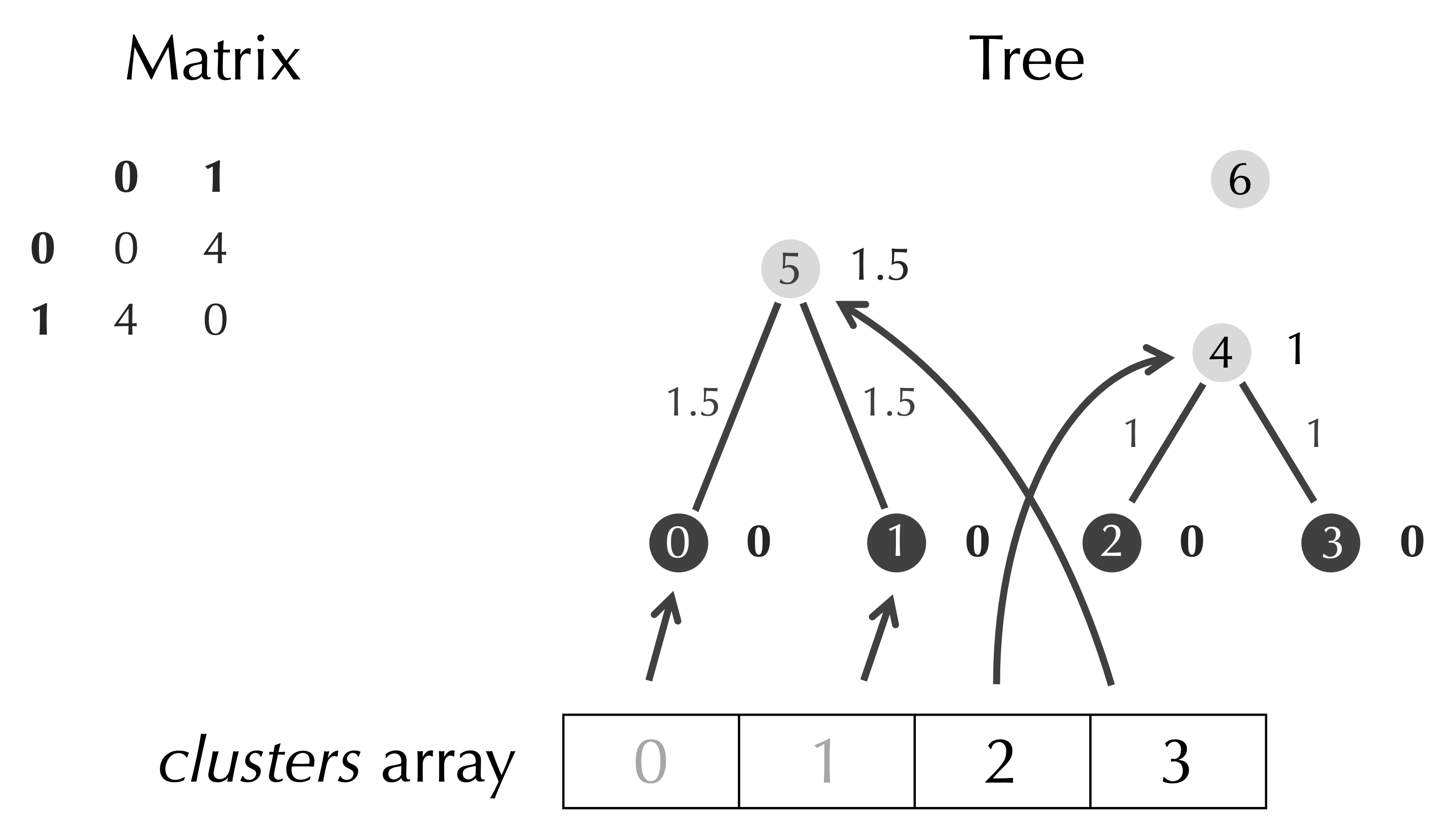
Next, we add a row and column to the matrix corresponding to the new node, and we gray out the rows and columns with indices row and col as they will be deleted.

We delete these rows and columns from the matrix, and we add a node to clusters that refers to our new node.

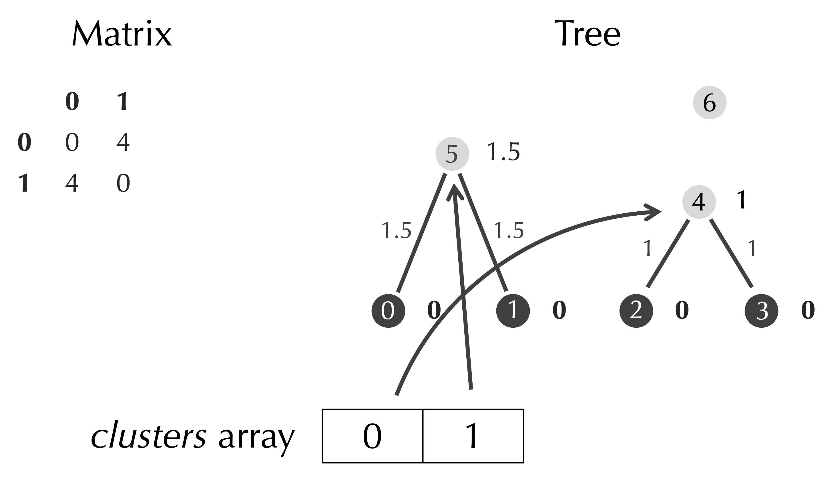
After deleting clusters[row] and clusters[col], we have completed another step of UPGMA.

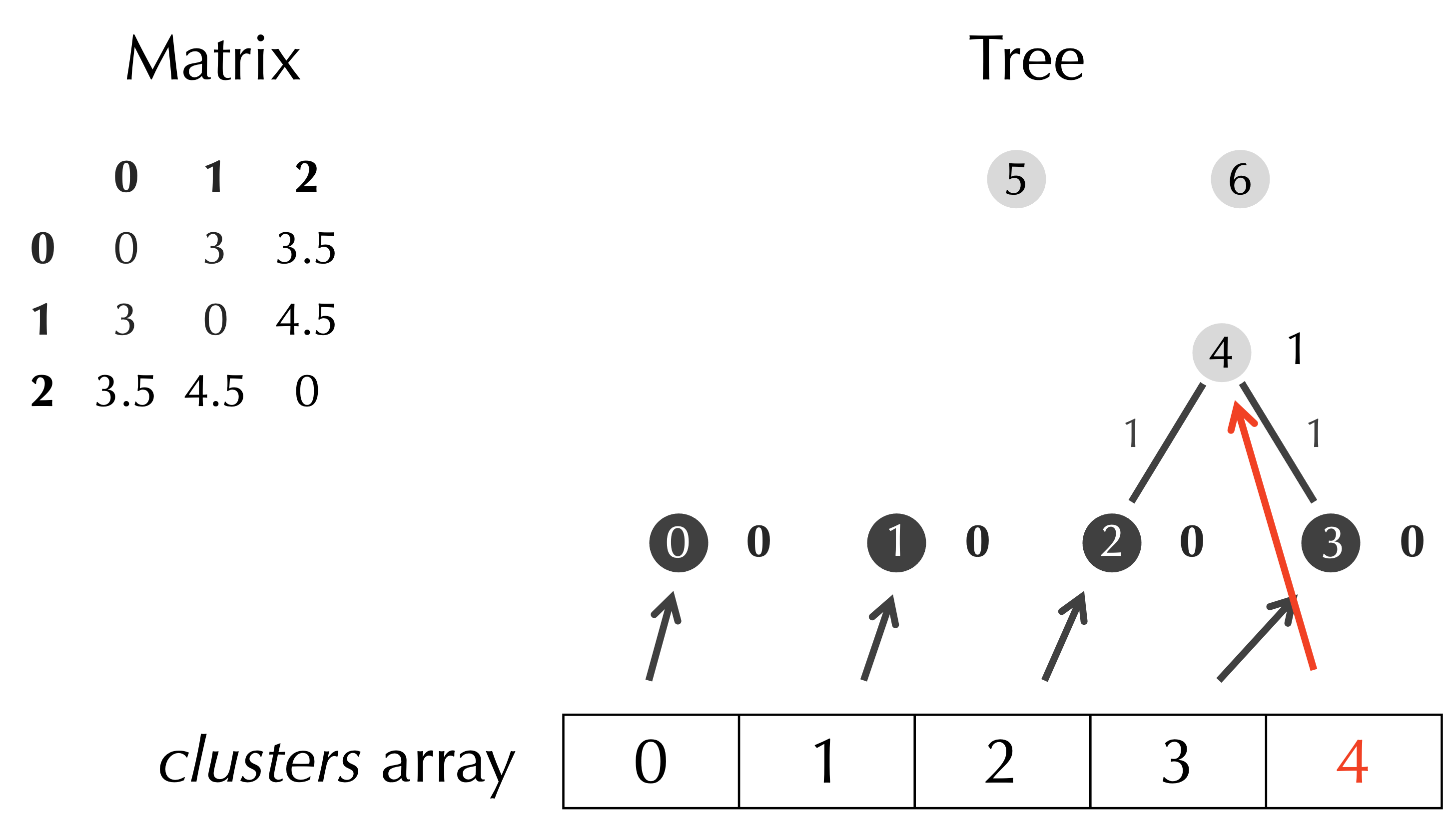
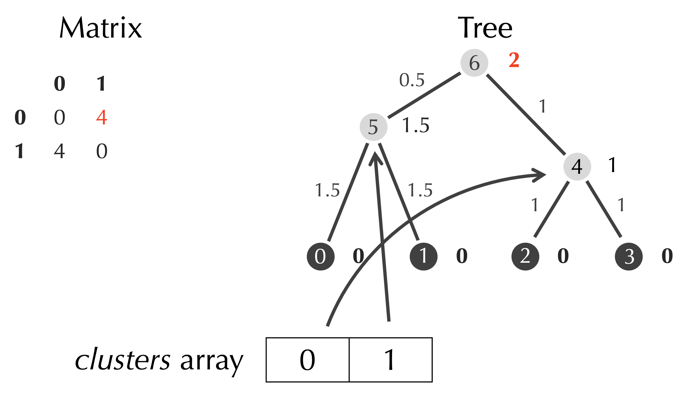
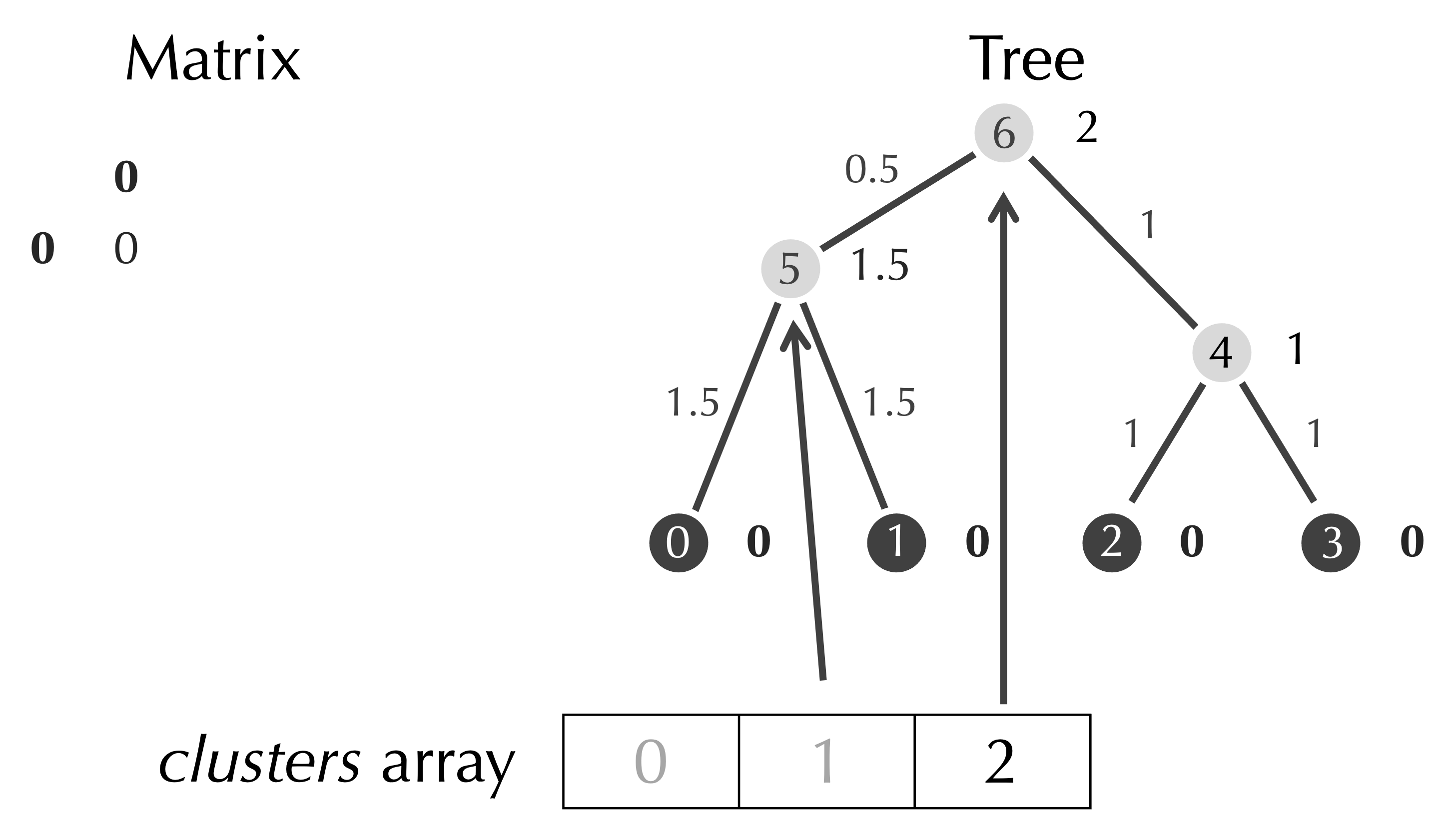
In our final step, we identify the minimum element of the matrix of 4, which occurs when row is 0 and col is 1. We assign half the minimum value, 2, as the age of the new node with index 6, and we connect this node to clusters[row] and clusters[col] via two edges.

When we add a row and column to the matrix, the only new value will be the distance from the new node to itself, which is zero.

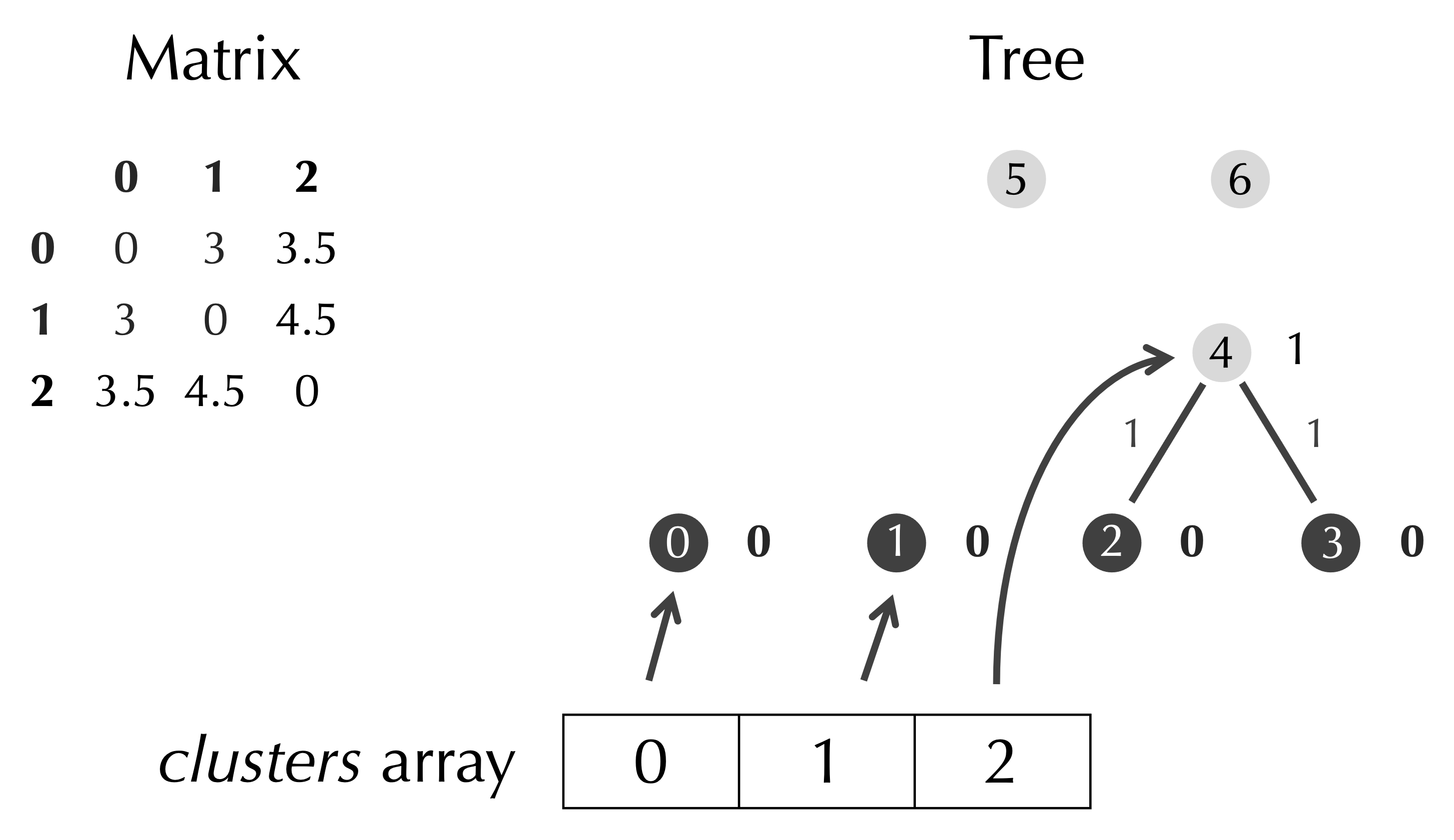
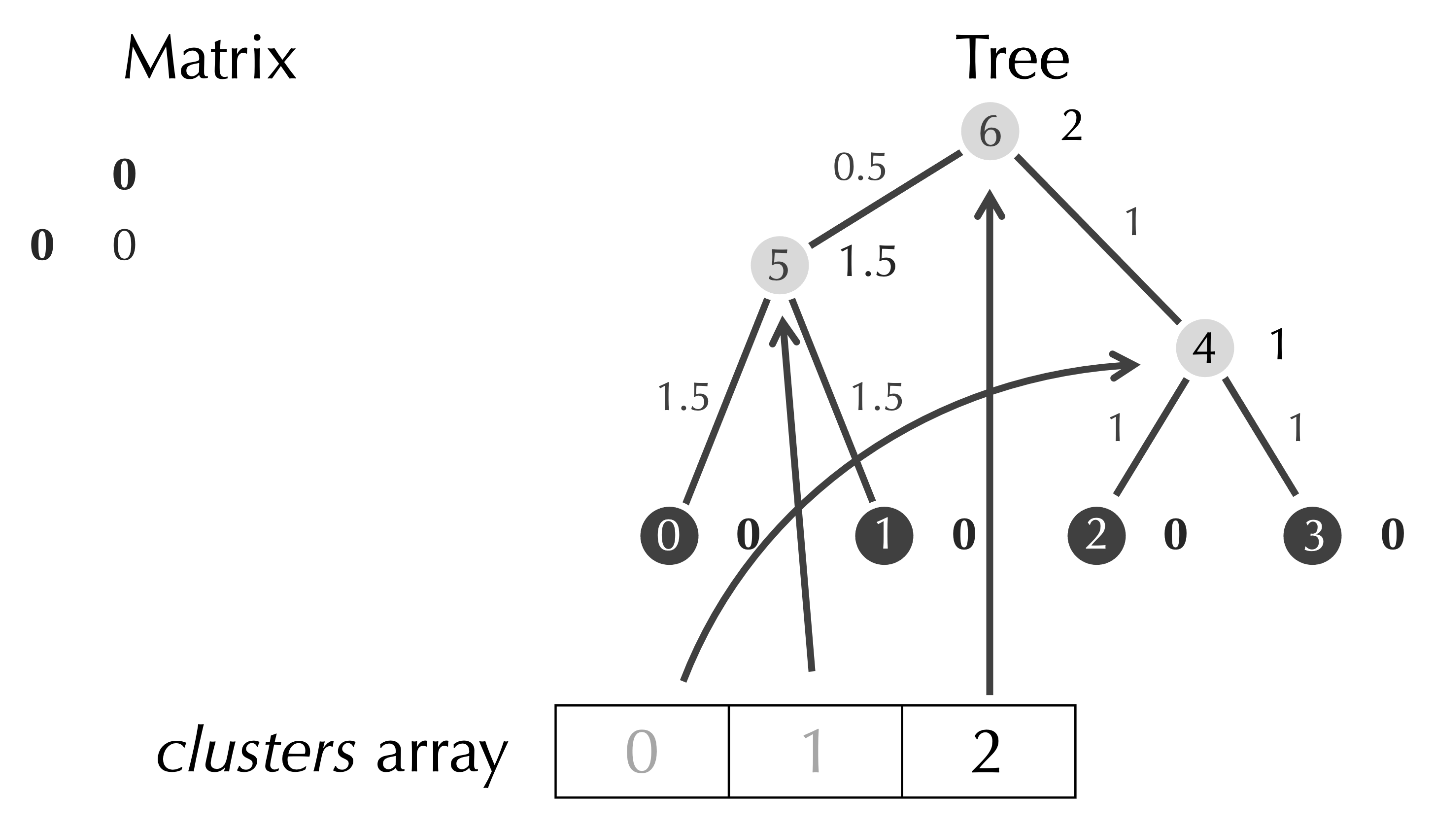
We remove the row and column of the matrix having indices row and col, and we add a reference in clusters that refers to our new node.

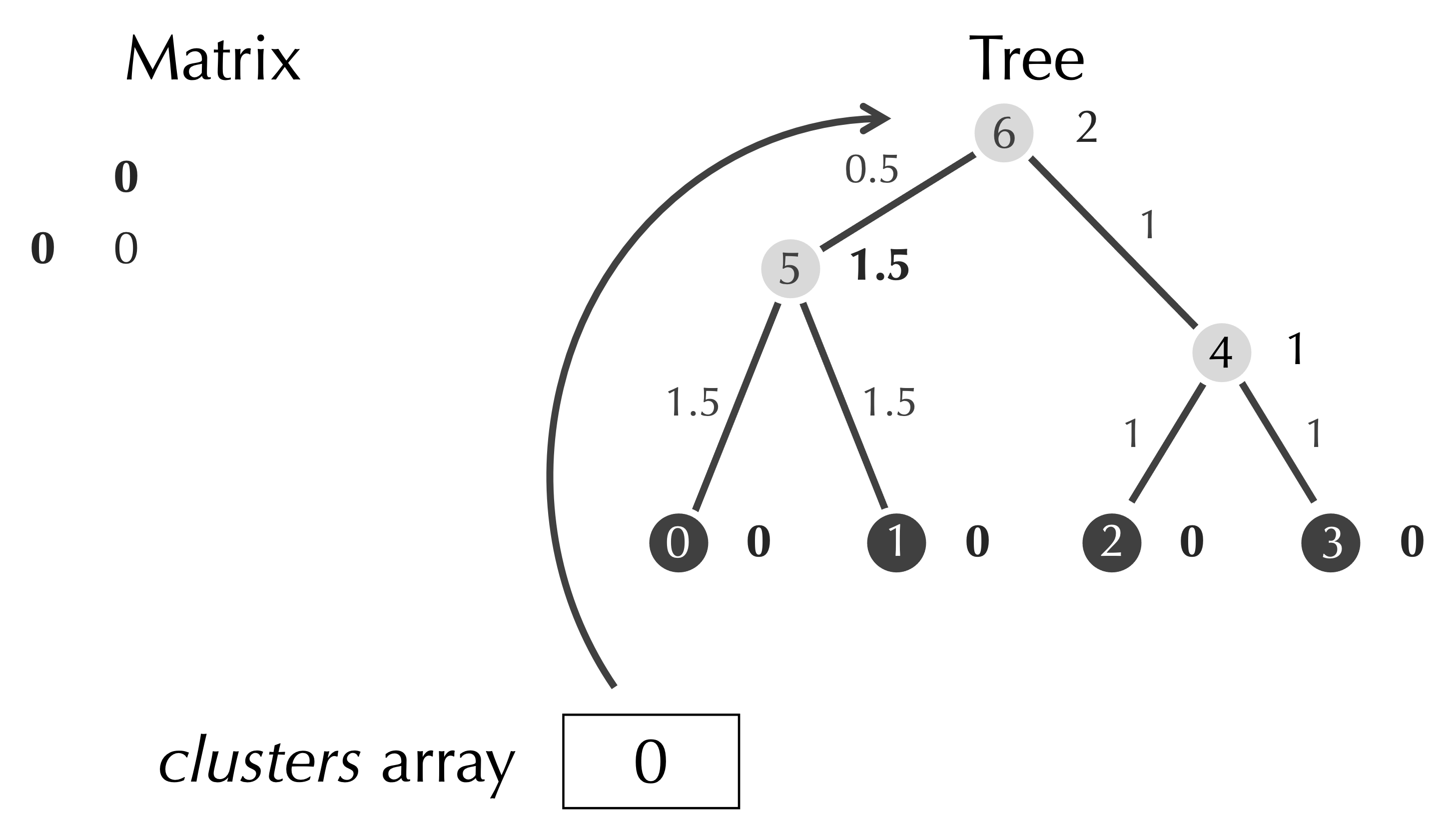
After removing clusters[row] and clusters[col], we have a matrix with only a single element, an array clusters with a single element referring to the root node of the tree, and a completed tree, which is the tree that we found before for this example.

Two subroutines needed for UPGMA

We have written our highest level function, and we should now focus on its subroutines. However, most subroutines called by UPGMA are short and would clutter our exposition here, and so we will discuss them in our code alongs. Two functions, however, are worth mentioning. First, we consider AddRowCol(), which takes as input a distance matrix D and integers row, col, clusterSize1, and clusterSize2. It returns the updated version of D with a new row and column, which are identical, and whose r-th element is equal to the weighted average of the distances D[row][r] and D[col][r]; these distances represent the distance from clusters[r] to each of the two clusters (clusters[row] and clusters[col]) that we are merging.

AddRowCol(D, row, col, clusterSize1, clusterSize2)
    newRow ← decimal array of length NumCols(D) + 1
    for every integer r between 0 and |newRow| – 2
        newRow[r] ← (clusterSize1 * D[row][r] + clusterSize2 * D[col][r] ) / (clusterSize1 + clusterSize2)
    D ← append(D, newRow)
    for every integer c between 0 and |newRow| – 2
        D[c] ← append(D[c], newRow[c])
    return D

Second, we consider CountLeaves(), which takes as input a Node object v, and returns the number of leaves “beneath” v (i.e., in the “subtree” of the UPGMA tree whose root is v). We have not yet encountered the special algorithmic approach needed to write this function, which we discuss in this chapter’s final section, which will complete our UPGMA algorithm and prepare us to implement it.