Ultrametric trees
The heuristic that we will adapt for evolutionary tree construction is called UPGMA, which stands for “Unweighted Pair Group Method with Arithmetic mean”. First published in 1958 by Sokal and Michener in the University of Kansas Science Bulletin (!), UPGMA helped launch the field of algorithms for evolutionary tree construction while also influencing clustering algorithms in modern machine learning.
In the previous lesson, we discussed unrooted trees. UPGMA produces rooted binary trees like the one shown in the figure below, which is a rooted version of an unrooted tree that we saw in the previous lesson. In a rooted binary tree, the root node has degree equal to 2, and every other internal node has degree equal to 3. As a result, we can think of time as proceeding downward on paths from the tree’s root to its leaves; every time we encounter an internal node on such a path, the tree branches into two additional nodes that are called the children of this node.
The rooted tree of primates in the figure below has the additional property of being ultrametric, which means that each node is labeled by a number called an age indicating its distance from the leaves. In the tree above, this number represents the age of the ancestor in millions of years; leaf nodes are all present-day species and receive an age of zero. UPGMA will produce an ultrametric tree.
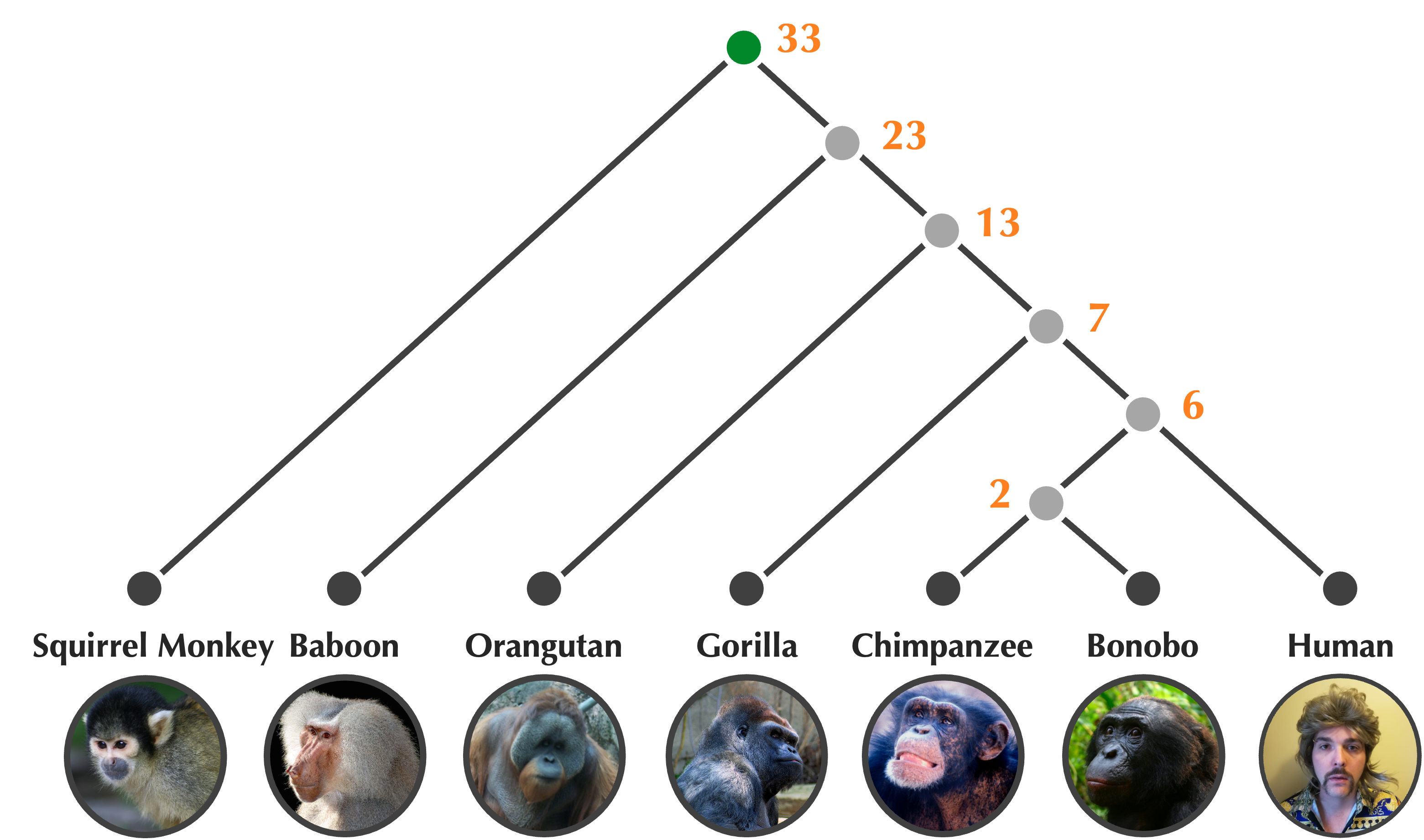
Once we have assigned ages to nodes in a rooted tree, we can obtain the edge weights for free by taking the absolute value of the difference between the ages of nodes that this edge connects. After we annotate the edges in this way, the updated tree (shown below) will have the property that all root-to-leaf path lengths are equal.

An overview of UPGMA
Consider the example distance matrix from the previous lesson reproduced below. Although this matrix has no tree fitting it precisely, we will walk through the steps UPGMA takes to produce a tree that fits it approximately. (In the next lesson, we will convert these ideas to pseudocode.)
| i | j | k | l | |
| i | 0 | 3 | 4 | 3 |
| j | 3 | 0 | 4 | 5 |
| k | 4 | 4 | 0 | 2 |
| l | 3 | 5 | 2 | 0 |
First, we form a leaf node for each element in our matrix.

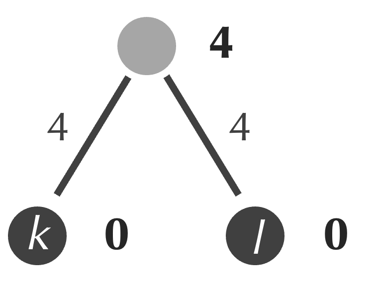
Next, although we saw in the previous lesson that this idea can sometimes lead us astray, we identify the minimum element of the matrix, which is equal to 2 and represents the distance between k and l. We form a new internal node connecting to both k and l, and we assign the age of this node equal to half of the matrix’s minimum value, or 1 (figure below). As a result, the edges connecting each of k and l to our new node receive weights equal to 1, which ensures that the path connecting k and l has length equal to 2.
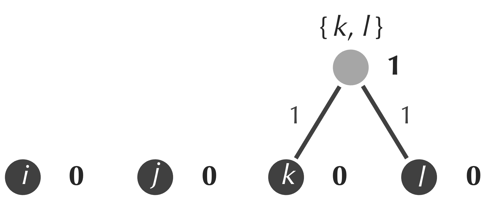
The formation of a new node serves as a merging of sorts, with k and l forming a new cluster that we represent as {k, l}. We can determine the distance from this cluster to i by averaging the distances D[i, k] and D[i, l] from the original distance matrix, which gives (3+4)/2 = 3.5. Similarly, we can compute the distance from {k, l} to j by averaging 4 and 5 to obtain 4.5. The table below shows the updated 3 × 3 distance matrix in which we perform this averaging to replace the rows and columns corresponding to k and l with a single row and column corresponding to {k, l}.
| i | j | {k, l} | |
| i | 0 | 3 | 3.5 |
| j | 3 | 0 | 4.5 |
| {k, l} | 4 | 4 | 0 |
distance matrix by merging k and l into a single element.
Now that we have a new distance matrix, we iterate the steps above. That is, we:
- find the minimum value of the distance matrix (3);
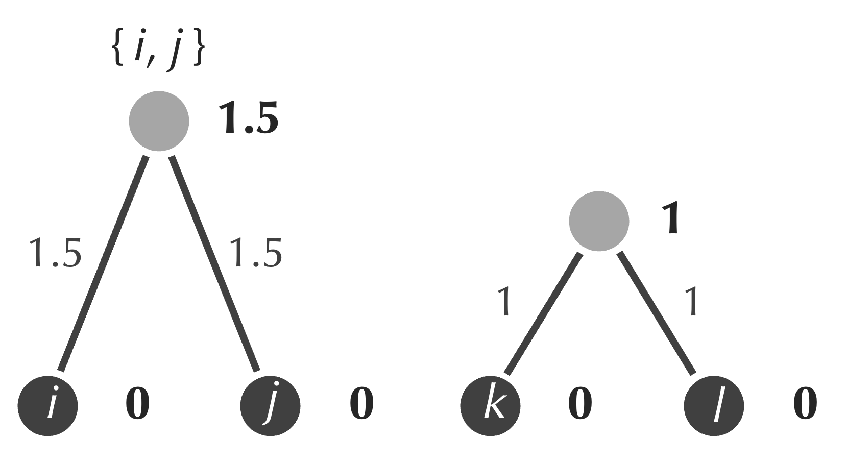
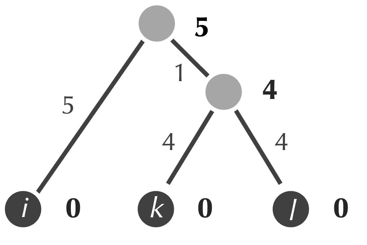
- form a new internal node connecting to the nodes corresponding to the minimum (i and j);
- assign the age of this node to be equal to half of the minimum value that we identified in the first step (1.5);
- assign weights of the two new edges to be equal to the differences between the ages of the new node and those of i and j (both are equal to 1.5);
- update the distance matrix by merging i and j to form a single element {i, j}, and setting its distance to each other cluster as the average of the distance from that cluster to each of i and j.
As a result of these steps, the updated tree is shown in the figure below.
The updated 2 × 2 distance matrix is shown below, in which the distance from {i, j} to {k, l} is equal to 4, the average of the distance from i to {k, l} (3.5) and the distance from j to {k, l} (4.5).
| {i, j} | {k, l} | |
| {i, j} | 0 | 3.5 |
| {k, l} | 4 | 0 |
Now that we have a 2 × 2 matrix, we apply the steps one final time:
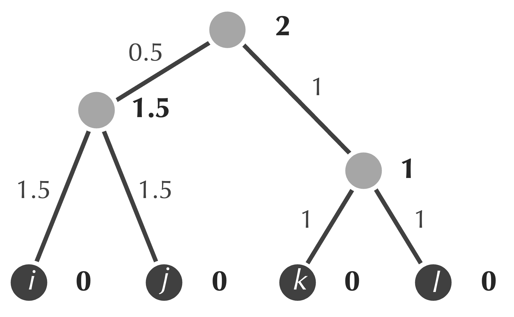
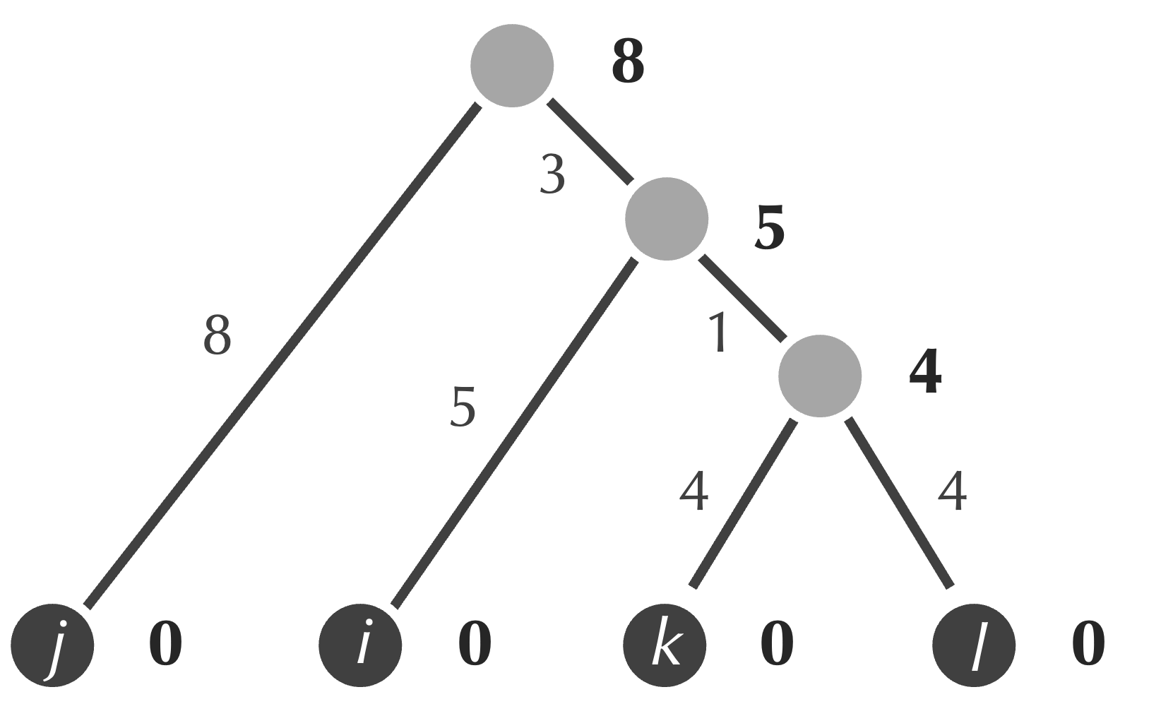
- find the minimum value of the matrix (4);
- form a new internal node connecting to the nodes corresponding to the minimum ({i, j} and {k, l});
- assign the age of this node to be equal to half of the minimum value that we identified in the first step (2);
- assign weights of the two new edges to be equal to the differences between the ages of the new node and those of {i, j} and {k, l} (equal to 0.5 and 1, respectively).
Once we have followed these steps, the final tree produced by UPGMA for this example is shown in the figure below. (Note that there is no need to update our distance matrix into a 1 × 1 matrix.)
UPGMA does not promise to fit a tree to a matrix
For the example above, we know that no tree exists fitting the matrix, and yet UPGMA has produced a tree. We should therefore pause to clarify that UPGMA will typically not produce a tree that fits a matrix, even if such a tree exists. For this example, note that the distances between leaf nodes in the tree produced by UPGMA sometimes match those in the matrix, and sometimes do not.
For example, consider our original matrix below.
| i | j | k | l | |
| i | 0 | 3 | 4 | 3 |
| j | 3 | 0 | 4 | 5 |
| k | 4 | 4 | 0 | 2 |
| l | 3 | 5 | 2 | 0 |
The tree produced by UPGMA is also reproduced below, with the path from i to l highlighted in red. This path has total length 4, but its corresponding distance matrix value D[i, l] is equal to 3. In general, the averaging performed by UPGMA means that for some pairs, the length of the path connecting them in the tree will be greater than the corresponding distance matrix value, and sometimes, this length will be lower than the corresponding distance matrix value.
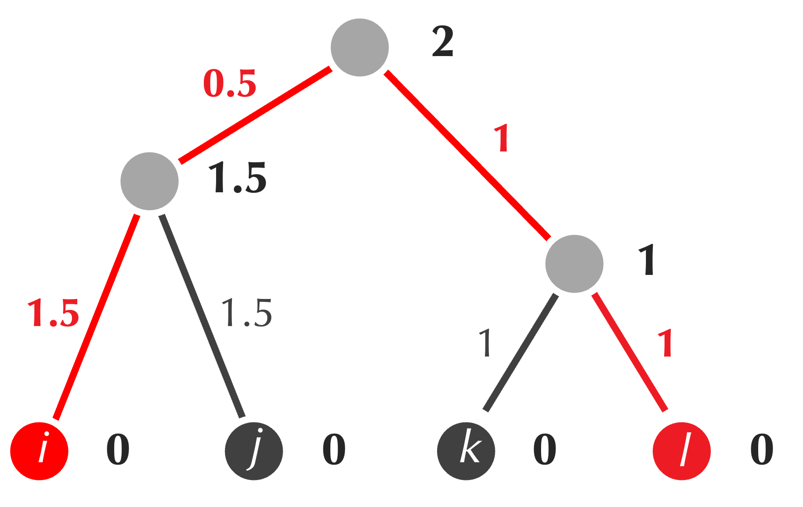
STOP: Which other pairs of leaves haven distances connecting them in the UPGMA tree that do not match the corresponding values in the original distance matrix?
Before we work on implementing UPGMA, we will give you an exercise allowing you to practice your understanding of the UPGMA algorithm.
Exercise: Apply UPGMA to the matrix shown in the figure below.
| i | j | k | l | |
| i | 0 | 20 | 9 | 11 |
| j | 20 | 0 | 17 | 11 |
| k | 9 | 17 | 0 | 8 |
| l | 11 | 11 | 8 | 0 |
Ensuring that averages are weighted
To check your work from the exercise above, we will show that after a single step, we identify that k and l should be merged, resulting in the tree and updated distance matrix below.
| i | j | {k, l} | |
| i | 0 | 20 | 10 |
| j | 20 | 0 | 14 |
| {k, l} | 10 | 14 | 0 |
one step of UPGMA to the distance matrix in the exercise
at the end of the preceding section.
After another step, we identify the minimum element of the matrix as the distance from i to {k, l}, and so we merge these two clusters. As a result, we obtain the updated tree and 2 × 2 distance matrix below.
| j | {i, k, l} | |
| j | 0 | 17 |
| {i, k, l} | 17 | 0 |
applying an additional step of UPGMA to the distance matrix
in the exercise at the end of the preceding section.
Unfortunately, this is wrong. If we consult the original matrix, then we see that the average distance from j to i, k, and l is equal to (20 + 17 + 11)/3 = 16, which conflicts with the value of 17 given above. So, what went wrong?
We computed the distance matrix value between j and {i, k, l} as 17 because it is the average of 20 (the distance from j to i) and 14 (the distance from j to {k, l}). However, the latter distance has already been computed as an average of two distances (D[j, k] and D[j, l] in the original matrix). The situation is comparable to an electoral process in which some constituents’ votes have greater impact than others, which obviously would be a bizarre thing to happen in a modern republic.
Note: The average that we are pointing out as incorrect is built into UPGMA’s sibling method, WPGMA (the “W” stands for “Weighted”). However, UPGMA is the vastly more successful algorithm since it produces averages without bias.
To avoid the bias caused by repeated averaging, we can weight the average that we compute. In this case, because {k, l} has two elements, we give the distance from j and {k, l} double the weighting when computing the average; that is, we compute the distance between j and {i, k, l} as (2 · 14 + 20)/3 = 48/3 = 16, as desired. This produces the correct 2 × 2 matrix shown in the table below.
| j | {i, k, l} | |
| j | 0 | 16 |
| {i, k, l} | 16 | 0 |
applying an additional step of UPGMA to the distance matrix
in the exercise at the end of the preceding section.
We have a 2 × 2 matrix, and so we can add the root to the tree and form the final tree produced by UPGMA below.
Now that we know how UPGMA works, we are ready to transition toward implementing it in the next lesson. You may like to think about what you have learned about object-oriented design to brainstorm what our objects should be for evolutionary tree construction and how we can convert the approach provided by UPGMA to pseudocode.