Reaction-Diffusion: Designing the Serial Engine in Python

Code along video

Learning objectives

We have reached the scientific heart of this chapter: a reaction-diffusion simulator. Particles of several species wander through a box by random walk, just like in our diffusion simulator, but now they can also react. When a predator and a prey wander close enough to each other, the prey may become a predator; a particle may also be born, die, or spontaneously change species. This model is the reason that we learned parallel programming in the first place, since checking which of thousands of particles are near each other is exactly the kind of heavy, large-scale work that rewards dividing it among many workers. In this lesson, we will tour the starter code (including a new object-oriented idea, inheritance), and then we will write the serial engine of the simulator, simulate_serial(), along with its helper rand_step(), which moves a particle and wraps it around the edges of the box.

Code along summary

Setup

To complete this code along, download the starter code as reaction-diffusion-python.zip (found here), expand the folder, and move the resulting reaction_diffusion directory into your python/src source code directory. The reaction_diffusion directory has the following structure.

• main.py: runs everything. It reads parameters from the command line, runs the serial and parallel simulations, animates each one, and prints how long each took and the resulting speedup. (Provided.)
• datatypes.py: our data classes, including particles, reactions, the reaction table, and the simulation parameters. (Provided.)
• custom_io.py: reads a reaction table from a CSV file and creates the initial particles. (Provided.)
• drawing.py, animate.py, and plotting.py: draw each frame with pygame, turn the frames into an MP4 movie, and plot the population of each species over time with matplotlib. (Provided.)
• serial.py: contains simulate_serial(), which we write in this lesson.
• functions.py: helper functions shared by the serial and parallel simulators. We write rand_step() in this lesson and the reaction functions in the next lesson.
• parallel.py: the parallel simulator, which we write in later lessons.
• data/: eight reaction CSV files (reactions_lotka_volterra.csv, reactions_rps.csv, reactions_rpsls.csv, reactions_sirs.csv, reactions_food_chain.csv, reactions_gause.csv, reactions_repressilator.csv, and reactions_gray_scott.csv).

Every function that we will write ourselves is already present in the starter code with its signature and a docstring explaining what it should do, followed by a pass statement. That way, the files can be imported from the start, and we fill in the bodies one at a time. The rendering code needs pygame, imageio, numpy, and matplotlib, all of which we have used in earlier chapters.

From Gray-Scott to individual particles

If you worked through the Gray-Scott practice exercises in an earlier chapter, then you have already seen a reaction-diffusion model. Gray-Scott zoomed out: each cell of a cellular automaton held concentrations of particles, cells exchanged concentrations with their neighbors (diffusion), and the concentrations changed according to simple rules (reactions). From these simple rules, beautiful Turing patterns emerged.

This time, we will zoom in. We will keep track of every individual particle, letting each one take random steps around the plane as in our diffusion simulator, and add reactions: rules saying what happens when particles meet. For example, a reaction might say that when a particle of species A (a predator) meets a particle of species B (its prey), the B particle becomes an A particle. The prey has been eaten, and we have one more predator.

Detecting exact collisions between moving particles would make our algorithm very slow, in any language. Instead, we adopt a simplification that scientists used back when computers had far less power. After the particles move, we check whether any two particles that could react are within some threshold distance of each other. If they are, the reaction fires with a probability given by the reaction’s rate. If the rate is 0.2, then we choose a random number between 0 and 1, and if it is smaller than 0.2, the reaction fires. So in addition to object-oriented programming and parallel programming, our simulator will rely on Monte Carlo simulation, and it brings together nearly everything that we have learned in this course.

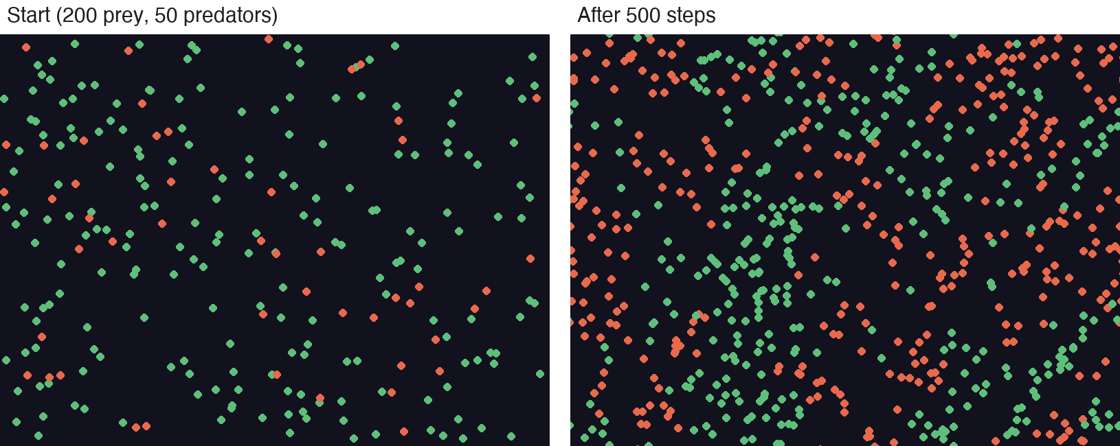
Our plan is the same as for diffusion: first we will implement the simulation serially, and then we will convert it into a parallel implementation that divides the box into vertical strips, one per worker. Recall that a parallel implementation can only beat a serial one under two conditions.

First, each worker must have enough nontrivial work to do, since setting up the workers has an overhead cost. In our diffusion simulator, a worker did little more than move points in random directions. Now, each worker will move points and check which pairs of particles in its strip are close enough to react, which is much more work. Second, we must solve the problem at a sufficient scale. Just as our parallel Monte Carlo simulation needed millions of trials rather than hundreds, we will need many hundreds or thousands of particles; if each of ten cores is responsible for ten particles, the parallel version has no hope of winning.

Dividing the space into strips also introduces a complication that diffusion did not have. A particle sitting near the border between two strips could react with a particle on the other side of that border, so the workers can no longer be completely independent. We will tackle that issue when we parallelize the simulator.

Particles and species

Let’s open datatypes.py. Our old friend OrderedPair stores an x and a y, and the Particle class is the one from our diffusion simulator with one new attribute. Each particle now has a species, an integer label. If our simulation has three species, then they are labeled 0, 1, and 2. Labeling species by integers means that we could have a simulation with 50 kinds of particles if we wanted to. The radius is used only for drawing, and the diffusion_rate is the length of each random step, so that a particle with diffusion rate 1 moves one unit in a random direction at each step. Recall that field(default_factory=OrderedPair) is the incantation that Python demands for an attribute whose default value is another object.

@dataclass
class Particle:
    """A single particle performing a 2D random walk.

    Attributes:
        position:       Current position as an OrderedPair.
        species:        Integer species ID (0-indexed, must be < num_species
                        in the reaction table).
        radius:         Visual radius (does not affect interactions).
        diffusion_rate: Length of each random-walk step.
    """
    position:       OrderedPair = field(default_factory=OrderedPair)
    species:        int         = 0
    radius:         float       = 5.0
    diffusion_rate: float       = 1.0

Reactions and inheritance

Next, we need to represent reactions. Every reaction proceeds at some rate, which we will interpret as a probability. For a reaction between two particles, the rate is the probability that the reaction happens when the particles are within the threshold distance. For a death reaction, a rate of 0.05 means that each particle of that species has a 5% chance of being removed in a given round of reactions.

But different kinds of reactions need different information. A reaction between two particles needs to know both species and what they produce; a death reaction only needs to know which species dies. This is where a principle of object-oriented programming called inheritance comes in. We declare a general Reaction class with a rate, and then we declare more specific classes that inherit from it by placing Reaction in parentheses after the class name. Each of these subclasses automatically receives the rate attribute and adds its own attributes.

@dataclass
class Reaction:
    """Base type for any reaction. All reactions carry a per-event rate.

    Subclasses add the species ids that participate. Reaction objects are
    plain data; the simulation loop discriminates on subclass.
    """
    rate: float


@dataclass
class ContactReaction(Reaction):
    """A reaction that fires when two particles come into contact.

    When a particle of species `catalyst` meets a particle of species
    `substrate`, the substrate becomes species `product` with
    probability `rate` per contact. The catalyst is unchanged.
    """
    catalyst:  int
    substrate: int
    product:   int


@dataclass
class UnaryReaction(Reaction):
    """A spontaneous (contact-free) species conversion.

    Each particle of species `from_species` converts to `to_species`
    with probability `rate` per simulation batch.
    """
    from_species: int
    to_species:   int


@dataclass
class BirthReaction(Reaction):
    """A spontaneous spawn of a new particle of `species` per batch."""
    species: int


@dataclass
class DeathReaction(Reaction):
    """A spontaneous removal of a particle of `species` per batch."""
    species: int

A ContactReaction involves two particles: a catalyst and a substrate. When they are close enough, the substrate is replaced by a particle of species product, and the catalyst is unchanged. If a predator (species 1) eats a prey (species 0) and produces a predator, then the catalyst is 1, the substrate is 0, and the product is 1. A UnaryReaction spontaneously converts one species into another, say from species 2 to species 1. A BirthReaction lets a particle of a species produce offspring with some probability, and a DeathReaction removes a particle with some probability.

This is the same idea as if we were building an early version of PowerPoint and returned to our shapes example. Rectangles and circles each have their own attributes, but they are all shapes, and so we could declare a Shape class holding what they share and let Rectangle and Circle inherit from it.

The reaction table and simulation parameters

The ReactionTable class gathers everything about the chemistry of a simulation. Its table attribute is a two-dimensional list in which table[i][j] is the ContactReaction that occurs when a catalyst of species i meets a substrate of species j, or None if those two species do not react. It also stores the number of species, a list of diffusion rates (diffusion_rates[i] is the step length of species i), a list of names (so that we can call species things like “Prey” and “Predator”), colors for drawing, a background color, and lists of the unary, birth, and death reactions. Most of the visual bulk of this class (shown below without its docstring) comes from field(default_factory=list), which gives each attribute a fresh empty list as its default.

@dataclass
class ReactionTable:
    table:            list[list[ContactReaction | None]] = field(default_factory=list)
    num_species:      int                                = 0
    diffusion_rates:  list[float]                        = field(default_factory=list)
    names:            list[str]                          = field(default_factory=list)
    colors:           list[tuple[int, int, int]]         = field(default_factory=list)
    background_color: tuple[int, int, int]               = (255, 255, 255)
    unary_reactions:  list[UnaryReaction]                = field(default_factory=list)
    birth_reactions:  list[BirthReaction]                = field(default_factory=list)
    death_reactions:  list[DeathReaction]                = field(default_factory=list)

Finally, SimulationParameters holds the global settings of the simulation. The particles live in a box of the given width and height, which we treat as a torus, as we did for diffusion: a particle that leaves through the top of the box re-enters at the bottom, and a particle that leaves through the right side re-enters on the left. The activation_range is the threshold distance within which two particles may react, and num_steps is the number of steps to run the simulation.

@dataclass
class SimulationParameters:
    """All fixed parameters governing the simulation.

    Attributes:
        width, height:        Box dimensions.
        num_particles:        Total particle count across all species.
        activation_range:     Distance within which conversion can occur.
        proximity_interval:   Number of motion steps between reaction checks.
        num_steps:            Total number of motion steps to run.
    """
    width:              float = 0.0
    height:             float = 0.0
    num_particles:      int   = 0
    activation_range:   float = 0.0
    proximity_interval: int   = 1
    num_steps:          int   = 0

The proximity_interval is the number of steps that the particles take between consecutive times that we apply reactions. Moving points is fast, but checking for reactions is expensive, especially in Python. And a single small step barely changes which particles are near a given particle, so we lose little by letting the particles take several steps before we look for reactions again.

The provided files and a reaction CSV

The other provided files contain no new ideas, which is why they are given to you for free. custom_io.py reads a reaction table from a CSV file. animate.py is the same file that we have used before to turn a list of pygame.Surface objects into a movie. drawing.py draws each snapshot of the particles to a surface, just as we drew boards and universes for cellular automata and the gravity simulator. plotting.py uses matplotlib to chart the number of particles of each species over time. And main.py parses the command line (which CSV to load, the box’s width and height, the number of steps), runs and animates the serial simulation and then the parallel simulation, and prints the timing of each along with the speedup.

Let’s look at the data in data/reactions_lotka_volterra.csv, which encodes the classic two-species predator-prey model named after Lotka and Volterra (the file’s comment lines are omitted below).

diffusion,0,1
diffusion,1,1
name,0,Prey
name,1,Predator
color,0,93,191,122
color,1,232,105,76
background,18,18,31
birth,0,0.026
death,1,0.026
1,0,1,0.1

The first two lines give the diffusion rates of species 0 and 1, the next two lines name them, and the color and background lines give RGB values for drawing. Prey (species 0) are born with rate 0.026, and predators (species 1) die with rate 0.026. The last line, which has four numbers, is a contact reaction: when a catalyst of species 1 (a predator) is within the activation range of a substrate of species 0 (a prey), the prey becomes species 1 with probability 0.1. The predator eats the prey, and we wind up with another predator. The other files in data/ use the same format to describe very different reaction systems, which we will explore at the end of the chapter.

Planning simulate_serial()

Our goal for the rest of this lesson is to write simulate_serial() in serial.py, the only function in this file. It takes a list of particles, a ReactionTable called table, and the SimulationParameters called params. It returns a list of snapshots, where each snapshot is a list of particles, which is the same pattern that we used for cellular automata and the gravity simulator.

def simulate_serial(particles: list[Particle],
                    table: ReactionTable,
                    params: SimulationParameters) -> list[list[Particle]]:
    """Run the simulation serially.

    Each batch:
      1. Move every particle proximity_interval times.
      2. Apply contact reactions once using the reaction table.
      3. Apply unary reactions (deaths, spontaneous conversions, births).
      4. Record a frame.

    Args:
        particles: Initial configuration (not mutated).
        table:     ReactionTable for conversion lookups.
        params:    Simulation parameters.

    Returns:
        List of snapshots, one per batch (including the initial step).
    """
    pass

The docstring lays out our plan. We group the steps of the simulation into batches. In each batch, every particle takes proximity_interval random steps; then we apply the contact reactions once, apply the unary reactions once, and record a snapshot (or frame).

As with diffusion, we begin by making a deep copy of the particles we are given, which we call current, so that we never change the caller’s list. We then create the list of frames that we will eventually return, whose first element is its own copy of the initial state.

# first, let's make the current list of particles and the list of "snapshots" that we eventually want to return
current: list[Particle] = copy.deepcopy(particles)
frames: list[list[Particle]] = [copy.deepcopy(current)]

return frames

Batches and leftover steps

How many batches (and therefore snapshots) will we have? Each batch contains proximity_interval steps, and so the number of batches is the total number of steps integer divided by proximity_interval. As we saw when dividing work among processes, an integer division usually leaves something left over, which we compute with the % operator.

# question: how many snapshots will I eventually take?
# remember: proximity_interval = number of steps between snapshots
num_batches = params.num_steps // params.proximity_interval
remainder = params.num_steps % params.proximity_interval

Now we range over the batches. Within each batch, we move every particle in current a total of proximity_interval times by calling a helper function rand_step(), which we will write shortly. We pass it the particle along with the box’s width and height, which it will need in order to wrap the particle around the edges of the box. We do not need the loop indices, so we use _ for both.

After the particles have moved, we apply the reactions. We split these into two functions, which we will write in the next lesson: apply_reactions() handles contact reactions between two particles, such as a predator eating a prey, and apply_unary_reactions() handles births, deaths, and spontaneous conversions. Both take the current particles, the table, and the parameters, and both return the updated list of particles, which we store back into current. Finally, we append a deep copy of current to frames.

After we range over all the batches, remainder steps are left over. We would probably never notice this bug if we skipped them, but to run the simulation for exactly num_steps steps, if remainder is positive, we move every particle remainder more times. The complete function is shown below.

def simulate_serial(particles: list[Particle],
                    table: ReactionTable,
                    params: SimulationParameters) -> list[list[Particle]]:
    """Run the simulation serially.

    Each batch:
      1. Move every particle proximity_interval times.
      2. Apply contact reactions once using the reaction table.
      3. Apply unary reactions (deaths, spontaneous conversions, births).
      4. Record a frame.

    Args:
        particles: Initial configuration (not mutated).
        table:     ReactionTable for conversion lookups.
        params:    Simulation parameters.

    Returns:
        List of snapshots, one per batch (including the initial step).
    """
    # first, let's make the current list of particles and the list of "snapshots" that we eventually want to return
    current: list[Particle] = copy.deepcopy(particles)
    frames: list[list[Particle]] = [copy.deepcopy(current)]

    # question: how many snapshots will I eventually take?
    # remember: proximity_interval = number of steps between snapshots
    num_batches = params.num_steps // params.proximity_interval
    remainder = params.num_steps % params.proximity_interval

    # now, I just range over all the batches and apply reaction-diffusion to each one
    for _ in range(num_batches):
        # move all my points proximity_interval times
        for _ in range(params.proximity_interval):
            for p in current:
                rand_step(p, params.width, params.height)

        # now I want to apply the reactions
        # contact reactions first, then unary
        current = apply_reactions(current, table, params)
        current = apply_unary_reactions(current, table, params)

        # add the current snapshot to overall list
        frames.append(copy.deepcopy(current))

    # we may have a few steps left over of just random walking
    if remainder > 0:
        # move all my points remainder times
        for _ in range(remainder):
            for p in current:
                rand_step(p, params.width, params.height)

    return frames

The imports at the top of serial.py (copy, our data types, and apply_reactions, apply_unary_reactions, and rand_step from functions.py) are already in the starter code. Notice that nothing here is new: we are combining ideas from diffusion with the object-oriented work of the last chapter, and passing the details of each step to subroutines.

Taking a random step on a torus

Now let’s write rand_step() in functions.py. We already wrote a function with this name in our diffusion simulator, so we copy its body from diffusion/functions.py. It chooses a random angle, and then it moves the particle by its diffusion rate times the cosine of the angle in the x-direction and the diffusion rate times the sine of the angle in the y-direction.

def rand_step(particle: Particle,
              width: float, height: float) -> None:
    """Take one random-walk step, wrapping around box edges.

    Args:
        particle: Particle to update (in-place).
        width:    Box width for wrapping.
        height:   Box height for wrapping.
    """
    angle = random.uniform(0.0, 2.0 * math.pi)
    particle.position.x += particle.diffusion_rate * math.cos(angle)
    particle.position.y += particle.diffusion_rate * math.sin(angle)

This is very close to what we want. The only difference is that our diffusion simulator never wrapped particles around the edges of the box, and so a particle could wander off the board. Rather than losing track of such a particle, or doing something complicated like bouncing it off the walls, it is much easier to treat the box as a torus. (If you completed the Gray-Scott exercises, you saw a flavor of this idea when cells at one edge of the grid had neighbors at the opposite edge.)

To wrap the particle, we first add the change in position to the current coordinate, and only after doing so, we take the result modulo the width (for x) or the height (for y).

def rand_step(particle: Particle,
              width: float, height: float) -> None:
    """Take one random-walk step, wrapping around box edges.

    Args:
        particle: Particle to update (in-place).
        width:    Box width for wrapping.
        height:   Box height for wrapping.
    """
    angle = random.uniform(0.0, 2.0 * math.pi)
    particle.position.x = (particle.position.x + (particle.diffusion_rate * math.cos(angle))) % width
    particle.position.y = (particle.position.y + (particle.diffusion_rate * math.sin(angle))) % height

Notice that rand_step() does not need to return anything. Python passes objects by reference, so when we pass a Particle into a function, the function has access to that very particle and can update its position directly.

Checking our work

We cannot run main.py yet, since apply_reactions() and apply_unary_reactions() are still stubs that return None, and so simulate_serial() would crash at its first batch. But we can test rand_step() on its own. Create a file check_rand_step.py in your reaction_diffusion directory that places a particle near the right edge of an 800 by 600 box and lets it take five steps. (We seed the random number generator so that the output is reproducible on your machine.)

import random

from datatypes import OrderedPair, Particle
from functions import rand_step


def main() -> None:
    """Walk one particle that starts near the right edge of an 800 x 600 box."""
    random.seed(4)
    p = Particle(position=OrderedPair(x=799.5, y=300.0), diffusion_rate=1.0)
    for _ in range(5):
        rand_step(p, 800.0, 600.0)
        print(p.position)


if __name__ == "__main__":
    main()

Running python3 check_rand_step.py shows the particle crossing the right edge of the box, reappearing on the left, crossing back, and crossing once more. Your numbers may differ from ours if your version of Python generates random numbers differently, but every x-coordinate should lie between 0 and 800.

OrderedPair(x=799.5875502040693, y=300.99616010850036)
OrderedPair(x=0.3847152191247005, y=301.5999216001274)
OrderedPair(x=799.590502402092, y=302.2075612970376)
OrderedPair(x=0.1527298717476242, y=303.0345439282728)
OrderedPair(x=1.0666622701257151, y=303.44041037329487)

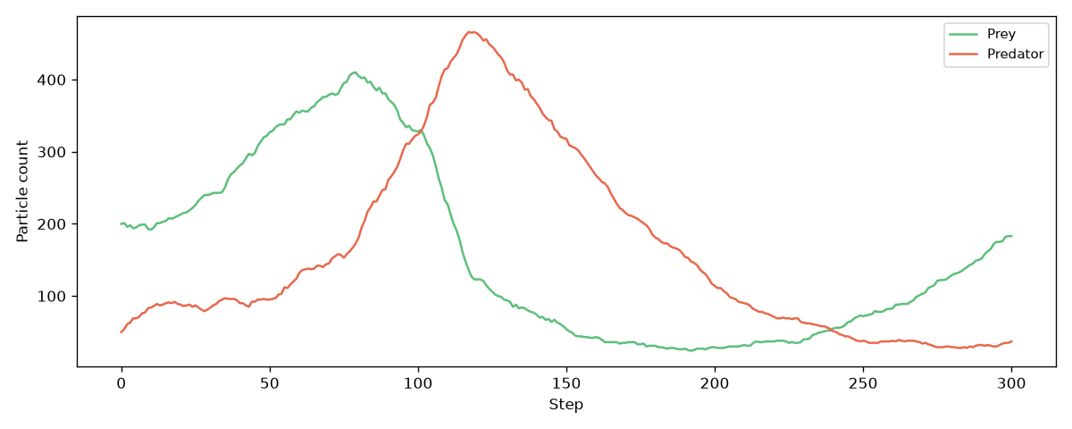
Once the reactions are in place, the simulator will produce population curves like the ones below, in which the prey flourish, the predators feast and multiply, the prey crash, and then the predators starve, allowing the prey to recover.

Looking ahead

Our serial engine is in place, but it relies on two functions that we have not yet written. In the next code along, we will implement apply_reactions(), which checks every pair of particles to see whether they are close enough to react, and apply_unary_reactions(), which handles births, deaths, and spontaneous conversions. Along the way, we will need to measure distance on a torus, which is a little trickier than it looks.