A Tour of Reaction Systems

Code along video

Learning objectives

Our parallel reaction-diffusion simulator is finished. In this final lesson of the chapter, we will put it to work. Each reaction system that we explore lives in its own CSV file of reaction rules, and the same simulator runs every one of them. We will tour predators and prey, competing species, an epidemic, a synthetic genetic oscillator, and rock-paper-scissors, and along the way we will see why parallelism matters: the simulations that tell the most interesting stories are the ones that would take far too long to run serially. We write very little new code in this lesson.

Code along summary

Setup

We will work in the reaction_diffusion folder that we completed in the previous lesson. Every reaction system in this lesson is a file in its data subfolder, so you do not need to download anything new.

Recall that main.py takes the way to place the particles (random scatters every species across the whole box, and clustered gives each species its own vertical band), a reaction file, the number of particles of each species, the width and height of the box, and the number of steps. For example, here is the first command that we will run.

python3 main.py random data/reactions_lotka_volterra.csv 500 1000 1000 50

Each run writes an animation (parallel.mp4) and a plot of the number of particles of each species over time (parallel_counts.png), along with serial versions of both until we turn the serial run off below, to a subfolder of output named after the reaction file. The figures on this page come from these runs; because our simulation is random, your pictures will differ in their details.

Reading a reaction file

Before we start our tour, let’s remind ourselves how a reaction file describes a system. Here is reactions_lotka_volterra.csv (minus the comments at the top).

diffusion,0,1
diffusion,1,1
name,0,Prey
name,1,Predator
color,0,93,191,122
color,1,232,105,76
background,18,18,31
birth,0,0.026
death,1,0.026
1,0,1,0.1

The diffusion, name, and color lines give each species (numbered starting at 0) its step length, its name, and its RGB color. The rest of the file holds the reactions.

A line of four values a,b,c,rate is a contact reaction: when a particle of species a comes within the activation range of a particle of species b, then with probability rate, the b particle becomes species c. In 1,0,1,0.1, a predator (1) that meets a prey (0) converts it into a predator with probability 0.1; that is, the predator eats the prey and reproduces.
birth,s,rate gives each particle of species s a probability rate of producing a new particle of the same species, placed randomly, every time we apply reactions. Because every prey particle gets its own chance, the more prey there are, the faster they reproduce.
death,s,rate gives each particle of species s a probability rate of disappearing.
spontaneous,s,t,rate gives each particle of species s a probability rate of turning into species t on its own, with no contact needed.

That’s all there is to it. Changing the system that we simulate means writing a new CSV file, not new code.

Predators and prey: the Lotka-Volterra model (2:30:09)

Our first system is a classic of ecology called the Lotka-Volterra model, which has two species: prey (green) and predators (orange). You can think of rabbits and wolves, or if you prefer, grass and rabbits. In plain language, the reaction file says three things.

When a predator meets a prey, it eats the prey (and makes another predator) with probability 0.1.
Prey reproduce on their own, so the more prey there are, the more new prey are born.
Predators die out on their own at a fixed rate.

In the video, Phillip first runs the model with 500 particles of each species in a 1000 by 1000 box for only 50 steps.

Note: In the video, this first run crashes with a TypeError inside apply_unary_reactions(): the birth rule was typed as if random.random < b.rate:, which compares the function random.random itself to a number. The fix is to call the function, if random.random() < b.rate:. If you followed our earlier lesson on applying reactions, then your code already has the parentheses.

After 50 steps, not much has happened; predators rise and prey fall, in both the serial and the parallel runs. Dynamics like these play out over thousands of steps, and so Phillip raises the number of steps to 250 and then to 1,500. At 1,500 steps, the serial simulation takes about 30 seconds, while the parallel simulation finishes in about two seconds, a speedup of roughly 15x on his 10-core machine.

STOP: If we keep increasing the number of steps, what happens to the time taken by the serial simulation? Is it still worth running the serial simulation at all once we trust our parallel one?

The serial simulator was valuable because it helped us check that the parallel simulator gives similar pictures. Now that we trust our parallel code, there is no reason to wait for the serial one. So Phillip turns off the serial part of main.py (2:35:58). He does this by wrapping the serial code in triple quotes, which first produces an IndentationError; a cleaner approach is to put a # at the start of each serial line (most editors do this for a selection with Cmd+/ or Ctrl+/). Remember to also comment out the lines at the end that print the serial time and the speedup, since they use serial_time. Here is how the middle of main() looks afterward.

# Run the serial simulator first, render its animation and counts plot,
# and time the simulation for comparison with the parallel version.
# print("Running serial simulation.")
# t0 = time.time()
# serial_frames = simulate_serial(particles, table, params)
# serial_time = time.time() - t0
# print(f"Serial simulation complete in {serial_time:.3f}s.")

# print("Rendering serial animation.")
# serial_surfaces = frames_to_surfaces(serial_frames, table, params)
# animate_surfaces(serial_surfaces, os.path.join(out_dir, "serial.mp4"))
# plot_species_counts(serial_frames, table, os.path.join(out_dir, "serial_counts.png"))

# Now run the parallel simulator (same inputs) so we can compare both
# the wall-clock and the resulting animations side by side.
print(f"Running parallel simulation ({num_procs} processes).")
t1 = time.time()
parallel_frames = simulate_parallel(particles, table, params, num_procs)
parallel_time = time.time() - t1
print(f"Parallel simulation complete in {parallel_time:.3f}s.")

print("Rendering parallel animation.")
parallel_surfaces = frames_to_surfaces(parallel_frames, table, params)
animate_surfaces(parallel_surfaces, os.path.join(out_dir, "parallel.mp4"))
plot_species_counts(parallel_frames, table, os.path.join(out_dir, "parallel_counts.png"))

print()
# print("--- Timing ---")
# print(f"Serial:   {serial_time:.3f}s")
print(f"Parallel: {parallel_time:.3f}s ({num_procs} processes)")
# if parallel_time > 0:
#     print(f"Speedup:  {serial_time / parallel_time:.2f}x")

If we rerun our 50-step command, the output now reports only the parallel simulation (your times will differ). You may also see a warning from imageio that the 1000 by 1000 frames are being resized to 1008 by 1008 for the video encoder; this is harmless, and the video shows it as well.

Reaction-diffusion simulation!
Loaded 2 species and 1000 particles.
Output: output/lotka_volterra/
Running parallel simulation (8 processes).
Parallel simulation complete in 1.220s.
Rendering parallel animation.
  Animation written to output/lotka_volterra/parallel.mp4  (11 frames @ 30 fps)
  Species count plot saved to output/lotka_volterra/parallel_counts.png

Parallel: 1.220s (8 processes)
Animation finished! Exiting normally.

With the serial simulation out of the way, Phillip runs the model for 4,500 steps, which takes about six seconds in parallel. The serial version would have taken several minutes.

python3 main.py random data/reactions_lotka_volterra.csv 500 1000 1000 4500

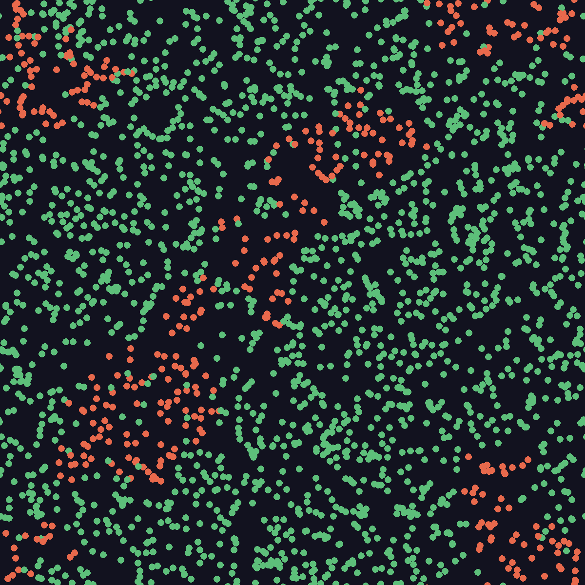
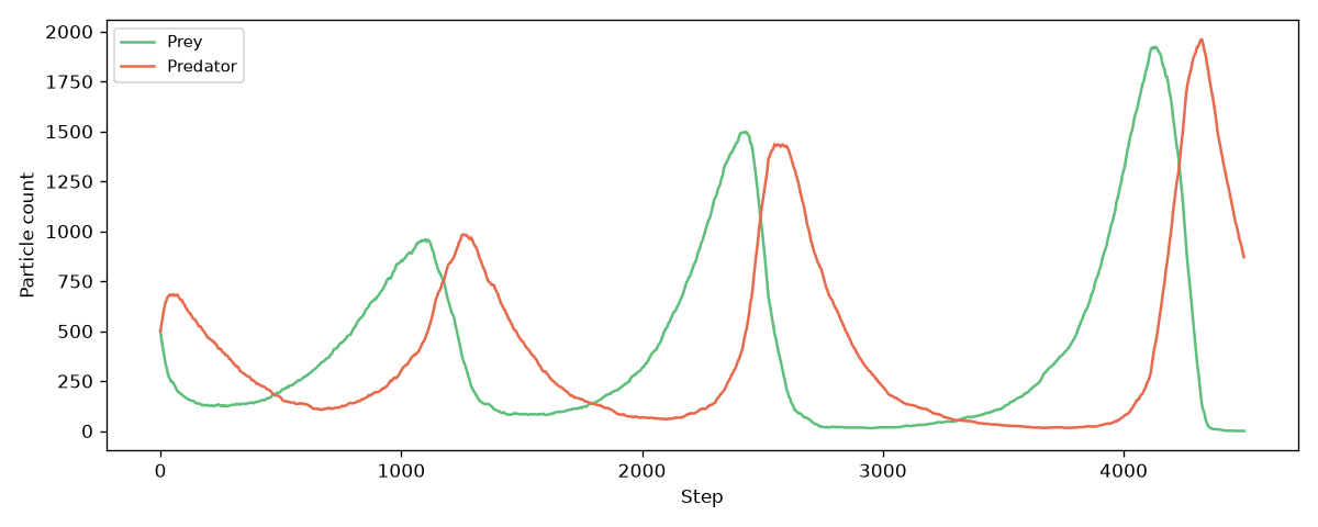
Snapshot of the Lotka-Volterra simulation: green prey particles fill most of the box, while narrow bands and clumps of orange predators eat their way into the prey — **Figure:** The Lotka-Volterra model after about 4,100 steps, near a peak in prey. Predators (orange) form fronts that sweep through the abundant prey (green).

Line plot of prey and predator counts over 4,500 steps; each prey peak is followed shortly by a predator peak, and the swings grow larger over time until the prey nearly vanish — **Figure:** Prey (green) and predator (orange) counts from a 4,500-step run. Each boom in prey is followed by a boom in predators, then a crash in prey, then a crash in predators. Notice that the swings grow over time.

The animation tells a story. When there are many rabbits, the wolves are happy, and their numbers rise. Soon the wolves cannot find enough rabbits, so the wolves die off, which lets the rabbits recover, and the cycle repeats. In the video’s run, the swings eventually grow so large that the rabbits run out entirely, and then the wolves, with nothing left to eat, die out too.

Alfred Lotka and Vito Volterra developed this model in the 1920s using differential equations, which produce smooth, predictable oscillations that continue forever. Those equations treat the populations as continuous quantities, but our simulation contains a finite number of individual particles that bump into each other at random. In a two-species system like this one, random chance pushes the populations from one cycle to a larger one, until some cycle swings so far that a population collapses. On a long enough time frame, somebody goes extinct. From a certain perspective, this is closer to real ecology, although the original equations remain foundational and have been applied to measured populations of real predators and prey.

Two predators, one food supply: Gause’s competitive exclusion (2:41:20)

Our next system comes from the biologist Georgy Gause, who studied competition about ten years after Lotka and Volterra. The model in reactions_gause.csv adds a second predator that eats the same food. We now have three species: a resource (green) and two competitors, A (blue) and B (orange).

The resource reproduces on its own.
When either competitor meets the resource, it eats it (and reproduces) with probability 0.1.
Both competitors die out on their own, and competitor B dies slightly faster than competitor A (rates of 0.03 versus 0.02).
The two competitors never interact directly; they compete only for food.

Phillip first starts each species in its own band with clustered, and competitor B dies out. Because he worries that the starting bands may have given blue an advantage, he reruns the system with every species scattered at random.

python3 main.py random data/reactions_gause.csv 500 1000 1000 4500

STOP: Before reading on, predict what will happen to the two competitors. Can they both survive on the same food supply?

Snapshot of the Gause simulation: a large patch of blue competitor A particles spreads through green resource particles, while a small cluster of orange competitor B particles sits near the bottom — **Figure:** The Gause model after about 3,000 steps, during a boom in the resource (green). Competitor A (blue) is spreading into the food, while competitor B (orange) holds on in one small cluster.

Line plot of resource, competitor A, and competitor B counts over 4,500 steps; the resource and competitor A rise and fall in two large boom-and-bust cycles, while competitor B stays small and disappears after about 3,500 steps — **Figure:** Counts for the Gause model. Competitor A (blue) feasts on each boom in the resource (green); competitor B (orange) gets only a small share and goes extinct.

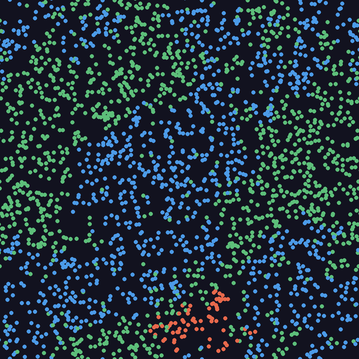
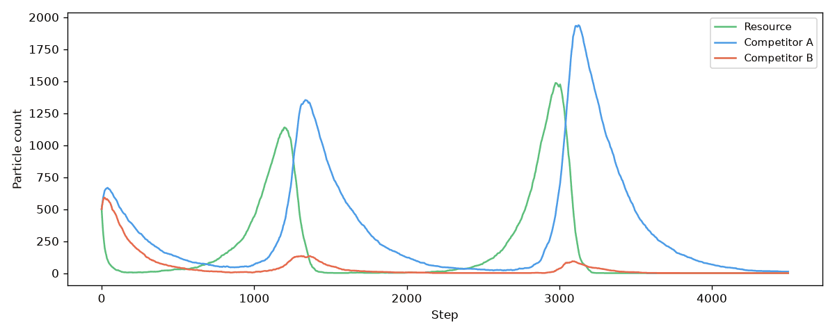
Both competitors start off nearly identical and scattered throughout the space, and yet one of them dwindles and disappears while the other survives in boom-and-bust cycles with the resource. In the video’s run, the orange competitor loses, and the same thing happened in ours. A slight edge at a key moment is enough: whichever competitor is a little more numerous when the food booms gets to feast on that boom, and the other falls further behind. (Later on, as in our predator-prey model, the noise can push the survivors into cycles so large that everyone collapses.)

This outcome is called the competitive exclusion principle: two species competing for exactly the same resource cannot coexist forever, and one of them drives the other to extinction. Gause verified the principle in the 1930s, and it has been confirmed with differential equations and many other models. It gives a mathematical reason why ecosystems are organized into niches: if two predators are going to share an environment, then they had better not eat the same food.

Epidemics: the SIRS model (2:47:23)

Our simulator is not limited to ecology. The same kind of rules describe how a disease spreads through a population, which is the subject of reactions_sirs.csv. Its three species are susceptible individuals (blue) who can catch the disease, infected individuals (orange), and recovered individuals (green).

When an infected individual meets a susceptible individual, it infects them with probability 0.1.
Infected individuals recover spontaneously, so this disease is not lethal.
Recovered individuals gradually lose their immunity and become susceptible again. (This is the final “S” in SIRS; the model without it is called SIR.)

python3 main.py random data/reactions_sirs.csv 500 1000 1000 4500

Snapshot of the SIRS simulation showing blue susceptible, orange infected, and green recovered particles mixed across the box, with small pockets of blue susceptible individuals surrounded by orange and green particles — **Figure:** A snapshot of the SIRS model after about 3,400 steps. Look for pockets of susceptible individuals (blue) surrounded by infected (orange) and recovered (green) individuals.

Line plot of susceptible, infected, and recovered counts over 4,500 steps; after an initial burst of infections, all three counts settle near an equilibrium and jitter around it — **Figure:** Counts of susceptible (blue), infected (orange), and recovered (green) individuals. After an early wave of infections, the system jitters around an equilibrium.

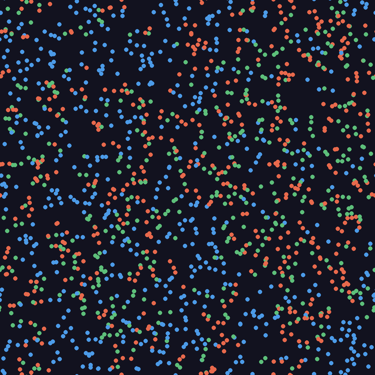
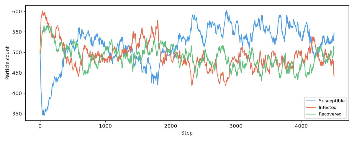
The counts show plenty of randomness, but everything moves toward an equilibrium in which the disease stays in the population. Every species diffuses with a step length of only 1, which reflects that people do not spread out wildly. The animation also shows a little bit of checkerboarding: pockets of susceptible people surrounded by infected or recovered people. This organization is not quite a Turing pattern, but it is undeniable, and patchiness like this is seen in real epidemics.

The purpose of this model is not to forecast a real epidemic. It is to show that one simulator that we built applies to a huge number of different situations.

Exercise: Add death to the SIRS model by creating a new reaction file in which infected individuals die with some small probability. Then explore reactions_food_chain.csv, which Phillip mentions in passing: wolves eat rabbits, and rabbits eat grass. Try python3 main.py random data/reactions_food_chain.csv 200,80,20 800 600 2000, where the comma-separated counts give a different number of particles for each species. How do the three levels of the food chain rise and fall relative to each other?

A genetic oscillator: the repressilator (2:49:29)

Oscillations are everywhere in biology. Your heartbeat is an oscillation, your circadian rhythm is an oscillation, and many cells contain oscillating chemical systems. Can a simple system explain how these oscillations arise? Around 2000, Michael Elowitz and Stanislas Leibler answered this question with the repressilator, a landmark of synthetic biology. They engineered a bacterium with three genes, each of which represses the next one in a cycle, and the bacterium’s proteins oscillated. (Our Biological Modeling course explores the repressilator in much more depth.)

Our file reactions_repressilator.csv names its three species after the genes in that circuit: lacI (light blue, which Phillip calls blue), tetR (yellow), and cI (pink). Each species “eats” the one that it represses.

0,2,0,0.15
1,0,1,0.15
2,1,2,0.15

When lacI (0) meets cI (2), the cI particle becomes lacI with probability 0.15.
When tetR (1) meets lacI (0), the lacI particle becomes tetR with probability 0.15.
When cI (2) meets tetR (1), the tetR particle becomes cI with probability 0.15.

These three rules form a cycle, and there are no births or deaths, so the total number of particles stays the same. Phillip first runs 500 particles of each species for 4,500 steps, and then he triples the number of particles.

python3 main.py random data/reactions_repressilator.csv 1500 1000 1000 1000

STOP: Every species starts with the same number of particles, placed at random. Do you think the three species will stay balanced? If not, in what order will they rise and fall?

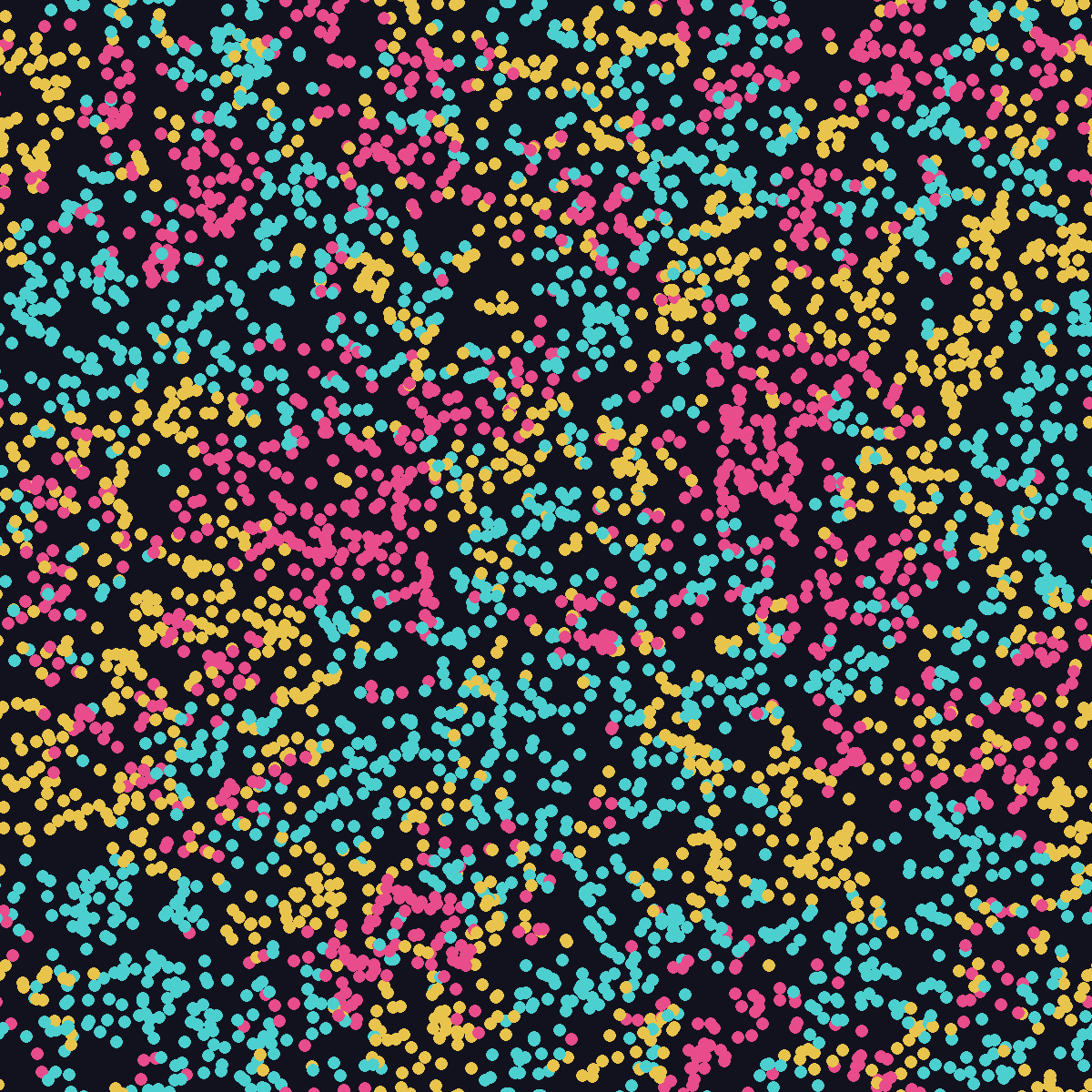
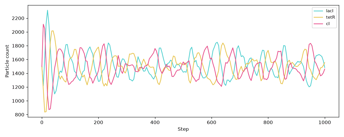
Snapshot of the repressilator simulation with light blue, yellow, and pink particles grouped into irregular patches of each color, with mixed colors along the borders between patches — **Figure:** The repressilator with 1,500 particles per species after about 625 steps. Particles that started at random have sorted themselves into patches of lacI (light blue), tetR (yellow), and cI (pink); reactions happen on the frontiers between patches.

Line plot of lacI, tetR, and cI counts over 1,000 steps; the three curves take turns peaking in a repeating order, oscillating between about 1,200 and 1,800 particles — **Figure:** Counts of lacI (light blue), tetR (yellow), and cI (pink) over 1,000 steps. A peak in cI is followed by a peak in lacI, then tetR, then cI again.

Even though the particles start at random locations, they quickly cluster into regions of each color, and the change in the system happens on the frontiers between regions, where we see waves and stripes that keep moving. Over time, the counts rise and fall in a fixed order: pink, then blue, then yellow, then pink again.

Why this order? When pink (cI) is abundant, it becomes food for the species that represses it. That species rises, since nothing holds it back, until the next species in the cycle finds a feast of its own. This is the same idea that drove the Lotka-Volterra model: when prey are abundant, their predators become abundant shortly thereafter. Two very different models, separated by about 75 years, rest on the same concept.

The peaks become sharper as we add more particles, because more particles means less randomness. Phillip pushes the system to 4,500 particles of each species (13,500 in all), which is close to the limit of what his laptop can handle. With that many particles packed into the box, the simulation needs some time to settle down before its oscillations take hold, and a larger box would be a better choice.

Rock, paper, scissors (2:57:05)

There is another way to sharpen the peaks: remove the randomness from the reactions themselves. If we take the repressilator’s reaction file and change every rate from 0.15 to 1.0, then every encounter between a predator and its prey results in the prey being converted. This is exactly reactions_rps.csv, which plays rock-paper-scissors in the plane: rock (gray) beats scissors (orange), paper (blue) beats rock, and scissors beats paper.

0,2,0,1.0
1,0,1,1.0
2,1,2,1.0

python3 main.py random data/reactions_rps.csv 1500 1000 1000 1000

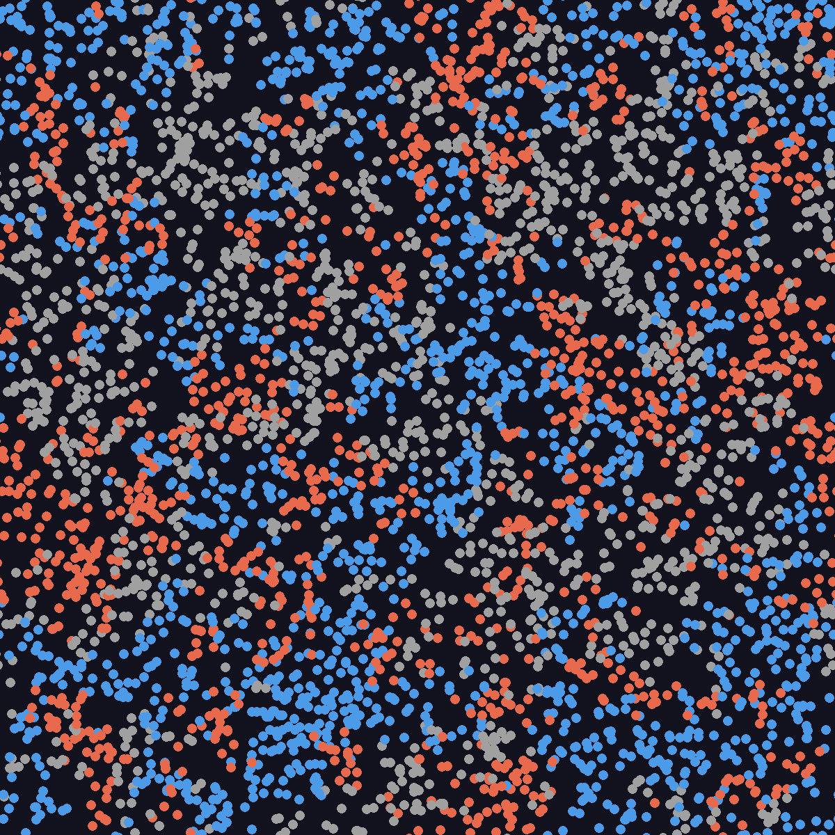
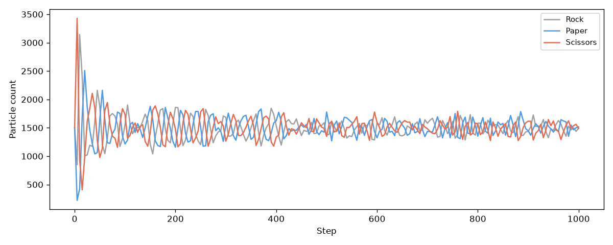
Snapshot of the rock-paper-scissors simulation with 4,500 particles: interleaved bands of gray rock, blue paper, and orange scissors cover the box — **Figure:** Rock-paper-scissors with 1,500 particles per species after about 825 steps: rock (gray), paper (blue), and scissors (orange) form interleaved fronts.

Line plot of rock, paper, and scissors counts over 1,000 steps; after large early swings, the three counts oscillate rapidly around 1,500 in a repeating order — **Figure:** Counts for rock-paper-scissors. With every reaction rate equal to 1.0, the species take turns peaking much faster than in the repressilator.

Because every encounter results in a reaction, the oscillations are much faster and the peaks are much sharper than for the repressilator. They come in a fixed order: scissors (orange), then rock (gray), then paper (blue), then scissors again. Rock comes right after scissors because rock beats scissors; when scissors are everywhere, every rock is surrounded by prey. It is a strange way of thinking about rock-paper-scissors, but it is equivalent. And all of this runs in parallel; there is no way that Phillip could have run this simulation live with the serial simulator.

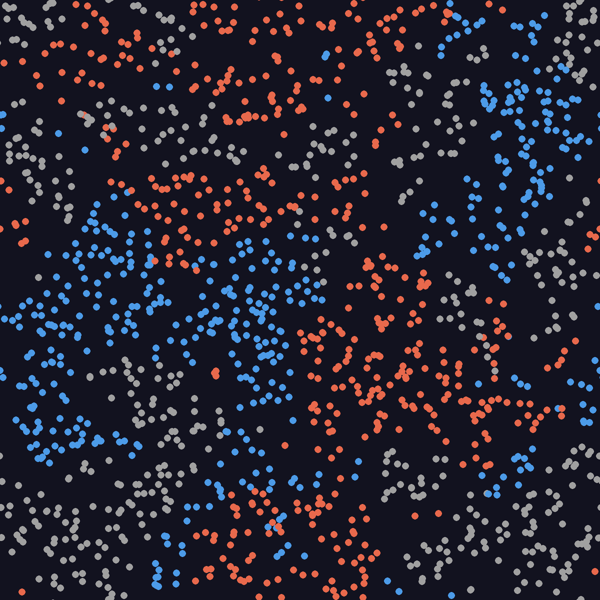
Phillip also reruns the model with fewer particles (500 of each species) started in bands with clustered. With fewer particles, we are back to more randomness, but stripes and spiraling fronts still emerge.

Snapshot of rock-paper-scissors started in bands with 500 particles per species: large regions of gray, blue, and orange particles curl around each other, with blue chasing gray, orange chasing blue, and gray chasing orange near the center — **Figure:** Rock-paper-scissors with 500 particles per species, started in bands, after about 325 steps. Each species chases its prey, and the fronts begin to curl around each other.

Rock, paper, scissors, lizard, Spock (3:01:14)

If we have rock-paper-scissors, then we are obligated to try rock-paper-scissors-lizard-Spock, a five-species extension made famous by the TV show The Big Bang Theory. Each species beats two others and loses to the remaining two, and every rate is 1.0.

Rock (gray) beats scissors and lizard.
Paper (blue) beats rock and Spock.
Scissors (orange) beats paper and lizard.
Lizard (green) beats paper and Spock.
Spock (purple) beats rock and scissors.

Phillip’s first run starts each species in its own band with 1,500 particles per species, and scissors wins almost immediately, taking over the whole box. Starting in bands means that each species initially meets only its neighbors, and the scissors band sat between paper and lizard, the two species that scissors beats. So Phillip scatters the particles at random instead. This run, with 7,500 particles, takes about a minute, and his computer’s fans let him know it.

python3 main.py random data/reactions_rpsls.csv 1500 1000 1000 1000

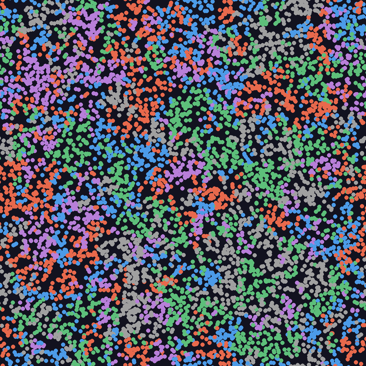
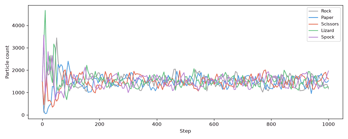
Snapshot of rock-paper-scissors-lizard-Spock with 7,500 particles: gray, blue, orange, green, and purple particles form overlapping stripes and patches — **Figure:** Rock-paper-scissors-lizard-Spock with 1,500 particles per species after 700 steps. Rock (gray), paper (blue), scissors (orange), lizard (green), and Spock (purple) still form radiating stripes.

Line plot of the five species counts over 1,000 steps; after wild early swings, all five hover between roughly 1,000 and 2,000 with no clear order of peaks — **Figure:** Counts for rock-paper-scissors-lizard-Spock. In our run, all five species survive, but the peaks are far less orderly than for three species.

Even with five species, we still see the same kind of radiating stripes. The peaks in the counts are much less clear than for rock-paper-scissors or the repressilator, because the system is more complicated, and we would need many more particles to see a clean alternation among five species. Often in this game, one or two strategies die out, leaving an ordinary game of rock-paper-scissors.

Exercise: Our simulator has plenty of parameters to play with. Choose one of the reaction files from our tour, copy it to a new file in data, and change one thing: a diffusion rate, a reaction rate, a birth or death rate, or a new reaction. Before you run it, predict how the counts plot will change, and then check your prediction. For example, what happens to rock-paper-scissors if rock diffuses twice as fast as the other two species?

Looking ahead

This concludes our chapter. We started with the idea of dividing work over many processors, learned to split a list, a Monte Carlo simulation, and a particle simulation across processes in Python, and then built a parallel reaction-diffusion simulator. In this lesson, that one simulator modeled predators and prey, competing species, an epidemic, a synthetic genetic circuit, and two playground games, and the parallel version let us run simulations in seconds that would otherwise take minutes. On a cluster with hundreds of cores, the same approach can turn a computation that would take days into one that takes minutes.

There is plenty more to try. You could add reactions that involve three particles at once, explore the remaining files in data such as reactions_gray_scott.csv (which aims at the Turing patterns that need a huge number of particles to appear), or invent a reaction system of your own. Phillip would love to see what you make, so share your animations on our Discord.

Back to Chapter 6