Code along video
Learning objectives
In this code along, we will turn from casinos to chemistry. Our goal is to build the engine of a diffusion simulator, in which many particles each take a random walk through a two-dimensional box. Before we can make this simulation run in parallel, we need a serial version that works, and so we will write simulate_serial(), which runs the simulation over many steps, along with two helper functions: update_particles(), which moves every particle one step and wraps it around the edges of the box, and rand_step(), which uses a little trigonometry to move a single particle in a random direction.
Code along summary
Setup
To complete this code along and the next one, download the starter code as diffusion-python.zip (found here), expand the folder, and move the resulting diffusion directory into your python/src source code directory. The diffusion directory has the following structure.
main.py: complete. It processes the command line arguments, places the particles withinitialize_particles(), runs and times the serial simulation and then the parallel simulation, renders each one to an MP4 video in anoutputfolder, and prints how much faster the parallel version was.datatypes.py: complete. Contains theOrderedPairandParticledataclasses.drawing.py: complete. Containsframes_to_surfaces()anddraw_frame(), which draw particles ontopygame.Surfaceobjects.animate.py: complete. Contains our old friendanimate_surfaces(), which writes a collection of surfaces to a video.serial.py: contains the signature and docstring ofsimulate_serial(), which we will write in this code along.functions.py: contains the signatures and docstrings ofupdate_particles()andrand_step(), which we will also write in this code along.parallel.py: contains the signatures and docstrings ofsimulate_parallel()andassign_stripes(), which we will write in the next code along.sine-and-cosine.png: a picture of the unit circle that will help us when we writerand_step().
You will need pygame, imageio, and numpy installed, just as when we animated our simulations in earlier chapters.
Diffusion as a random walk
In the previous code along, we parallelized a Monte Carlo simulation of craps. Now we will apply the same ideas to a simulation of particles. We will model the diffusion of a single particle through space as a random walk: at every step, the particle picks a direction uniformly at random and moves a fixed distance in that direction. We will do this for many particles at once, which is where parallelism will eventually come into play, since every particle follows its own random walk independently of the others. Over time, the particles spread out.
Open main.py. The usage of our program is as follows.
python3 main.py <num_particles> <num_steps> <width> <scatter|center> <drawing_frequency>
The parameters tell the program how many particles to simulate, how many steps to run, how wide the box should be (in pixels, since we draw the box at its native size), where the particles start, and how many steps should pass between consecutive frames of the animation. With center, every particle starts in the middle of the box, like a drop of dye placed in a glass of water. With scatter, the particles are placed uniformly at random throughout the box.
Most of main.py is code that we have written many times before: it parses command line arguments, runs our serial simulation and renders it, and then runs our parallel simulation and renders it. It relies on initialize_particles(), which takes the number of particles, the width and height of the box, the radius of each particle, how far a particle moves in a single step, and whether to scatter the particles. It returns a list of Particle objects placed in the box. You are welcome to read it, but there is nothing earth-shattering here.
Data types
Open datatypes.py. We have an OrderedPair dataclass that we have seen before, whose x and y attributes default to zero. A Particle has a position, which is an OrderedPair; recall that when an attribute of a dataclass is an instance of a user-defined class, we need to use field(default_factory=OrderedPair) so that every particle gets its own position. A particle also has a radius, which is used only for drawing, and a diffusion_rate, which is the length of the step that the particle takes in each generation.
@dataclass
class OrderedPair:
    x: float = 0.0
    y: float = 0.0


@dataclass
class Particle:
    position:       OrderedPair = field(default_factory=OrderedPair)
    radius:         float       = 5.0
    diffusion_rate: float       = 1.0
The drawing code in drawing.py and animate.py is nearly identical to what we have used before. frames_to_surfaces() takes our list of frames (each frame is its own list of particles), the size of the box, a background color, a particle color, and a drawing frequency, and it calls draw_frame() to produce a pygame.Surface for every frame that we want to draw. Then animate_surfaces() converts these surfaces into a video, with the help of a surface_to_numpy() subroutine.
Writing simulate_serial()
Open serial.py. The function simulate_serial() takes our initial list of particles, the number of steps (generations) to run, and the width and height of the box. Why does the simulation need to know the size of the box? When a particle flies off one side of the box, we will have it reappear on the other side. If a particle exits through the bottom, it comes back in at the top, and if it exits on the left, it comes back in on the right.
The fancy way of saying this is that we are simulating our particles on a torus, which is the surface of a donut. If you walk all the way around a donut in either direction, you wind up back where you started.
This function should feel familiar, since it follows the same pattern as the cellular automata and gravity simulators that we have written before. We create a list frames whose elements are lists of particles, one for each time point of the simulation. Its first element is a copy of the initial particles, which we make with copy.deepcopy() so that we have a completely fresh collection of data, with every attribute of every particle copied over. Then we range from 1 up to and including num_steps, appending the result of updating the previous generation, and at the end we return frames.
    def simulate_serial(particles: list[Particle],
                        num_steps: int,
                        width: float,
                        height: float) -> list[list[Particle]]:
"""Run the simulation serially, recording every step.

Args:
    particles: Initial configuration (not mutated).
    num_steps: Total number of random-walk steps to run.
    width:     Box width (used for periodic wrapping).
    height:    Box height (used for periodic wrapping).

Returns:
    List of snapshots of length num_steps + 1 (including step 0).
"""
        # let's create a list of (lists of particles) corresponding to the time points of our simulation
        frames: list[list[Particle]] = [copy.deepcopy(particles)]

        # range over all the steps and update the universe
        for i in range(1, num_steps+1):
            frames.append(update_particles(frames[i-1], width, height))

        return frames
STOP: Why does our loop start at 1 instead of 0, and why does it stop atnum_steps+1? How many lists of particles willframescontain when the function returns?
Moving every particle on a torus
Next, open functions.py, which will hold helper functions that both our serial and our parallel simulations can call. The function update_particles() takes the current list of particles along with the width and height of the box, and it returns a new list of particles in which every particle has taken one step in a random direction, with a length equal to its diffusion rate.
Since we are producing a new list of particles, we start by making a deep copy of the current list. Then we range over the particles in the new list and move each one in a random direction by calling a subroutine rand_step(). Note that we call rand_step(p) without setting p equal to anything; because p refers to an instance of a user-defined class, the function can change the particle’s attributes directly.
After a particle moves, it may have stepped off the side of the board, in which case we need to wrap it around. This is where the remainder operator saves the day. If the box has width 10 and a particle’s x-coordinate becomes 11, then 11 % 10 is 1, so the particle reappears one unit from the left side. And in Python, the remainder operator works in the other direction too, since the remainder of a negative number divided by a positive one is always nonnegative.
>>> 11 % 10
1
>>> -1 % 10
9
>>> -0.25 % 10.0
9.75
We can therefore write p.position.x = p.position.x % width, or, more compactly, p.position.x %= width. This is the first time that we have used the %= operator, but it works just like +=. We do the same for the y-coordinate, using the height of the box, and then return the new list.
    def update_particles(current: list[Particle],
                         width: float,
                         height: float) -> list[Particle]:
"""Advance every particle by one random-walk step on a torus.

After each random-walk step, particle positions are wrapped modulo
the box dimensions, so the simulation lives on a periodic domain
(a torus): a particle leaving the right edge re-enters from the left.

Args:
    current: Particle list at the current step (not mutated).
    width:   Box width (used for periodic wrapping in x).
    height:  Box height (used for periodic wrapping in y).

Returns:
    A fresh particle list with each particle moved one step,
    with positions wrapped into [0, width) x [0, height).
"""
        new = copy.deepcopy(current)

        # range over all the particles and update their positions
        for p in new:
            rand_step(p)  # move in a random direction
            # it may be the case that we stepped off the side of the board, in which case we want to wrap around
            p.position.x %= width
            p.position.y %= height

        return new
Note: In the video, Phillip typesp.position.y %= width, and he catches the mistake in the next code along. Becausemain.pyalways uses a square box, the slip does no harm in practice, but the y-coordinate should be wrapped by the height of the box, as shown above.
It may have sounded fancy that we are implementing our simulation on a toroidal surface, but at the end of the day, the torus amounts to just these two lines of code. They are the only place where wrapping appears in our program, because we have passed all of the remaining work of moving a particle to rand_step().
STOP: If you implemented a simulation of boids in an earlier chapter, did it wrap around the edges of the screen? How many lines of code did you need to do it?
Moving a single particle with a little trigonometry
Finally, we need rand_step(), which takes a particle, moves it a distance equal to its diffusion rate in a random direction, and returns nothing. If the diffusion rate is high, the particle moves a lot in each step; if it is low, the particle barely moves.
The easy part is choosing the direction. We pick an angle uniformly at random between 0 and 2π using random.uniform(). The angle needs to be in radians, because the trigonometric functions in the math module assume that angles are given in radians.
The harder part is knowing how far to change the particle’s x- and y-coordinates. Here is where a little trigonometry comes in handy. If we move a distance of 1 at an angle θ, then the change in x is cos(θ) and the change in y is sin(θ), as shown in the figure below. This holds regardless of the value of θ, in any quadrant. And if we move a distance r instead, then the changes become r · cos(θ) and r · sin(θ).
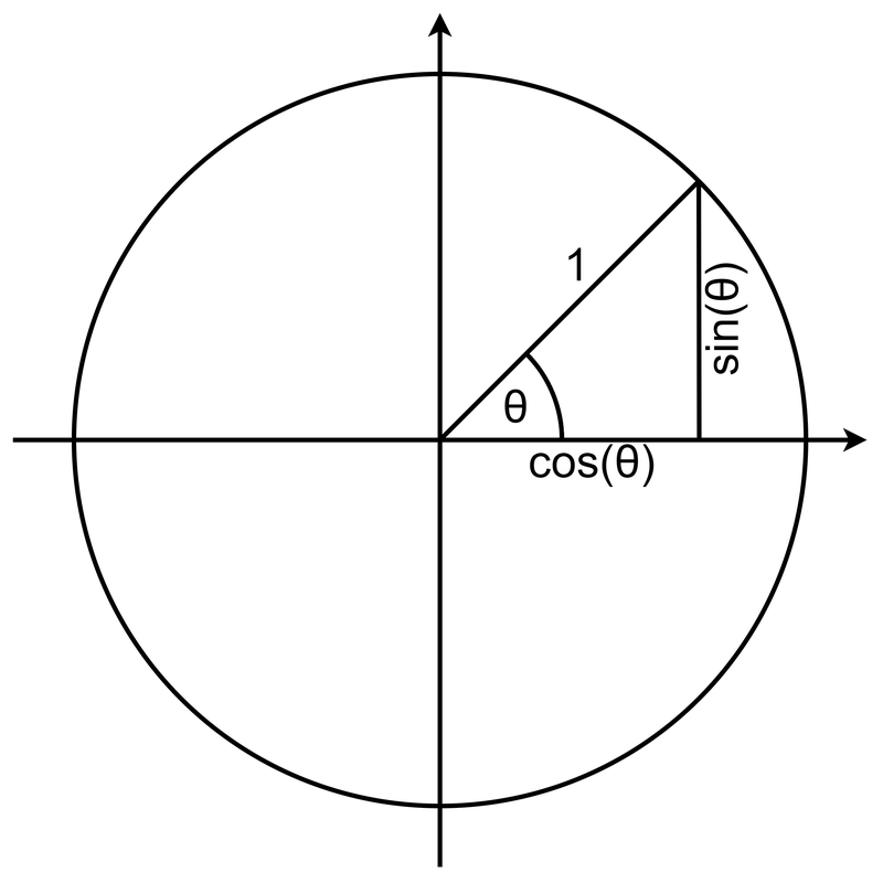
So we add particle.diffusion_rate * math.cos(angle) to the particle’s x-coordinate and particle.diffusion_rate * math.sin(angle) to its y-coordinate. That is all three lines of code that we need, and we do not need to return anything, since the particle that we were given has been moved.
    def rand_step(particle: Particle) -> None:
"""Move a particle by its diffusion rate in a uniformly random direction.

Args:
    particle: Particle to update (in-place).

Returns:
    None
"""
        # pick a random direction of motion as an angle in rads
        angle = random.uniform(0.0, 2.0*math.pi)

        # then, we want to update the x and y coordinates of the position of particle
        # we know that we are moving a length equal to particle.diffusion_rate
        particle.position.x += particle.diffusion_rate * math.cos(angle)
        particle.position.y += particle.diffusion_rate * math.sin(angle)
Note: In the video, Phillip typesmath.Piwith a capital P. Python names are case sensitive, and themathmodule has no attribute calledPi, so this line raises anAttributeErrorthe first time the simulation runs, which happens in the next code along. The constant ismath.pi, as shown above.
Our serial simulation in action
And that is it for our serial simulation. In each generation, every particle moves in a random direction according to its diffusion rate, and if it flies off the board, we wrap it around to the other side. That didn’t take too long!
We cannot run python3 main.py from start to finish just yet, because main.py also calls simulate_parallel(), which we will write in the next code along. To test our work, we ran simulate_serial() on 1,000 particles starting in the center of a box of width 300 for 1,000 steps, and then we drew every tenth frame with the functions in drawing.py and animate.py. The figure below shows four frames of the resulting animation: the drop of dye spreads out over time, just as we expected.
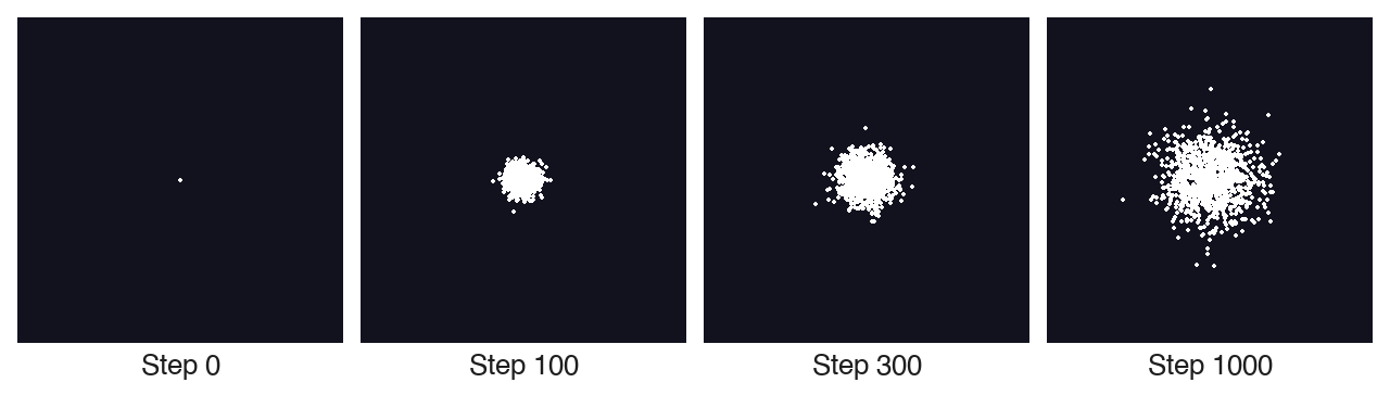
STOP: As the particles spread out, the cloud grows. Do you think that the width of the cloud grows in proportion to the number of steps? For example, will the cloud after 1,000 steps be ten times wider than it was after 100 steps? (Hint: compare the frames in the figure above.)
Exercise: Each particle in this simulation is independent of the others, so we can learn a lot by following just one. Write a functionaverage_squared_distance()with signaturedef average_squared_distance(frames: list[list[Particle]], step: int, start: OrderedPair) -> float:that returns the average, over all particles inframes[step], of the squared distance from the particle’s position tostart. Then simulate 1,000 particles starting at the center of a box of width 1000 withdiffusion_rateequal to 1, and print the result for steps 100, 200, 400, and 800. What pattern do you notice? (Use a box that is wide enough that no particle wraps around, or your distances will be thrown off.)
Looking ahead
Our serial diffusion simulator works, but it updates every particle one at a time, even though no particle cares what any other particle is doing. In the next code along, we will write simulate_parallel(), which divides the box into vertical stripes, hands each stripe of particles to its own worker, and uses a Pool and its starmap() method to update all of the stripes at once. Then we will finally run main.py and see whether our parallel simulation is any faster than our serial one.