Parallel Diffusion with Pool and starmap in Python

Code along video

Learning objectives

In this code along, we will parallelize our diffusion simulator. We will see why the Process and Queue approach that served us so well for craps is a disaster when the workers need new instructions at every step, and we will replace it with a pool of workers that is created once and reused. We will divide our torus into vertical stripes, hand each stripe to a worker with pool.starmap(), combine the results, and retire the workers with pool.close() and pool.join(). Finally, we will time our serial and parallel simulations against each other and ask why the parallel one is slower.

Code along summary

Setup

We will continue working in the diffusion folder from the previous code along, where our serial simulator is finished; this time, we will replace the pass statements in the two functions of parallel.py, simulate_parallel() and assign_stripes().

The shape of a parallel simulation

Our parallel simulator has the same overall shape as simulate_serial(). It takes the initial list of particles, the number of steps, and the width and height of the board, and it returns a list of generations, each of which is a list of particles. The only new input is num_procs, the number of workers that we will use. Here is the function signature and docstring that you will find in parallel.py, which already imports copy, multiprocessing, Particle, and update_particles().

def simulate_parallel(particles: list[Particle],
                      num_steps: int,
                      num_procs: int,
                      width: float,
                      height: float) -> list[list[Particle]]:
    """Run the simulation by splitting particles into spatial stripes.

    Each step:
      1. Assign current particles to num_procs vertical stripes by x.
      2. pool.starmap advances every stripe by one random-walk step.
      3. Reassemble into a global frame.

    Args:
        particles: Initial configuration (not mutated).
        num_steps: Total number of random-walk steps to run.
        num_procs: Number of worker processes (= number of stripes).
        width:     Box width (for striping and periodic wrapping).
        height:    Box height (for periodic wrapping).

    Returns:
        List of snapshots of length num_steps + 1 (including step 0).
    """

We begin the same way as before. We make a deep copy of the input particles that we will call current, which will hold the current generation and update as we go. Then we make our list of frames, whose first element is a second, independent deep copy of current.

# current will store my current generation of particles
current = copy.deepcopy(particles)
frames: list[list[Particle]] = [copy.deepcopy(current)]

Why our craps paradigm fails here

When we parallelized craps, we followed five steps: make a queue to store results, create the worker processes, start them, join them, and then grab and combine everything in the queue. It is very tempting to drop those five steps straight into the loop that we wrote for our serial simulation, so that at every step of the simulation, we split up the particles among a collection of workers.

# important point to be made

for i in range(1, num_steps+1):

    # 1. create a queue to store our results
    # 2. initialize our worker processes
    # 3. start the processes, which will put their return values into the queue
    # 4. range over all processes and "join" them (wait until all are finished before continuing)
    # 5. grab all results from the queue and combine

return frames

Before we go any further, let’s make the parallelization strategy precise. The natural way to divide this work is to divide the space: every worker is responsible for one equally sized stripe of the board, and if a particle lands in your stripe, you are responsible for moving it.

When we implemented craps in parallel, we had one queue and one worker per core. Here, we would create a new queue at every step, and far worse, we would create a new set of processes at every step, for a total of num_steps * num_procs processes. If we run 10,000 steps on a machine with 10 cores, that is 100,000 processes, each of which must be set up and torn down, and each of which only moves a handful of particles one tiny step before it disappears.

We know from craps that processes come with overhead. That overhead is fine when each process does a lot of work, as when every craps worker played many thousands of games and reported back once. But in diffusion, every worker needs new instructions at every step, and the result is comical. When Phillip tried this approach, a simulation that took about 0.04 seconds serially took about 34 seconds in parallel.

A pool of workers created once

Our solution is to keep the stripes but create the workers once, at the very start, so that we only ever have num_procs workers. The tool for this is a pool, which we create with multiprocessing.Pool(num_procs). A pool is a collection of workers that persist across many different tasks. In our Monte Carlo simulation, each worker received one task (play a lot of games and report back). Here, we will give the same workers a fresh set of instructions at every step, like players in a game whose rules change every round.

We could make the pool smaller or larger than the number of processors, but the natural choice is one worker for each processor that we want to use. Once the pool exists, we range over the steps, and at each step we divide the space into stripes using a subroutine assign_stripes() that we will write shortly. It takes the current particles, the number of workers, and the width of the board, which it needs in order to know how wide each stripe is. For example, if we have 10 workers and a board of width 100, then each stripe has width 10.

# it would be a bad idea to create workers every time through a new generation

# each worker is going to be responsible for a vertical "stripe" of our space of equal size
# the workers are only going to get initialized once (create a pool)
pool = multiprocessing.Pool(num_procs)

# range over all the steps
for _ in range(1, num_steps+1):
    # divide the space
    stripes = assign_stripes(current, num_procs, width)
    # stripes[0] holds the particles associated with worker 0, stripes[1] holds particles for worker 1, etc.

return frames

Here, stripes is a list of lists of particles: stripes[i] holds the particles that worker i is responsible for at the current step.

Handing out work with starmap

Next, we assign each worker exactly one stripe and tell all of them to get to work. We do this with the pool’s starmap() method, which needs two things. The first is the function that every worker should call, which for us is update_particles(), the serial function that we wrote in the previous code along and that parallel.py already imports from functions.py. This is the beauty of a coherent parallel design: each worker runs ordinary serial code, ranging over its own particles and moving each one a random step. There is nothing parallel about update_particles() itself.

The second thing that starmap() needs is the arguments for each worker’s call. Since update_particles() takes three parameters (a list of particles, the width, and the height), each worker needs a tuple of three values. Note that every worker needs the width and height of the whole board, and not just its stripe, because a particle that flies off the edge of the board must wrap around to the other side. So we build a list worker_args whose length is the size of the pool and whose i-th element is the tuple of arguments for worker i.

# next, assign each worker precisely one stripe

worker_args: list[tuple[list[Particle], float, float]] = []

# let's assign the i-th worker the three parameters that update_particles needs
for stripe in stripes:
    worker_args.append((stripe, width, height))

# this starts the process of each worker calling update_particles() on its stripe (subset of particles that it was assigned)
moved_stripes = pool.starmap(update_particles, worker_args)

# the starmap call blocks until they are all finished

# in other words, we wait on them to all finish

That type hint on worker_args is quite a mouthful, but it is about as good an argument for type hints as we will ever find. Writing worker_args = [] would be shorter, and Python would not complain, but it would leave a reader (including you, a week from now) guessing at what goes in the list. The hint says exactly what each worker receives: a list of particles, a float for the width, and a float for the height. Note also the double parentheses in worker_args.append((stripe, width, height)), since we are appending a single tuple.

If you have used Python’s pool.map() before, you may wonder why we need starmap(). The function map() passes each element of the list as a single argument, which only works when the function takes one parameter. Because update_particles() takes three parameters, we need starmap(), which unpacks each tuple into separate arguments (the “star” refers to Python’s * operator for unpacking).

Calling pool.starmap() starts every worker on its stripe, and it blocks until all of them are finished. This is exactly what we want: we should not combine the workers’ results until every worker has reported back, so we can only be as fast as our slowest worker. Notice also that we no longer have to manage a queue; the pool collects each worker’s return value behind the scenes, and starmap() returns them as a list in the same order as worker_args.

Combining the results

Since update_particles() returns a list of particles, moved_stripes is a list of lists of particles, where moved_stripes[i] holds the particles that worker i moved. To rebuild the current generation, we start current as an empty list and add each moved stripe to the end of it.

You might reach for current.append(stripe), but append() would add the whole list as a single element. To add the elements of one list to the end of another, Python provides extend(). Once we have combined all the stripes, we have the updated positions of every particle, and we append a deep copy of current to frames.

# let's combine their work
current = []

# at this point in time, moved_stripes is a list[list[Particle]] where moved_stripes[i] has the particles that were moved by worker i

for stripe in moved_stripes:
    # stripe is a list[Particle]
    current.extend(stripe)

# we now have updated positions of all particles and I will add the current snapshot into frames

frames.append(copy.deepcopy(current))

The order changes, because particles are now grouped by stripe. Since we only ever draw the particles and never track an individual particle by its index, this does no harm.

Retiring the workers

Once the loop over steps is finished, we let the workers go. We do this with two calls: pool.close() tells the pool that no more work is coming, and pool.join() waits for the worker processes to exit. In other contexts, join() would wait for the workers to finish their last tasks, but we already know that they are all finished, because starmap() blocked until they were. Finally, we return the frames. Here is our finished simulate_parallel().

def simulate_parallel(particles: list[Particle],
                      num_steps: int,
                      num_procs: int,
                      width: float,
                      height: float) -> list[list[Particle]]:
    """Run the simulation by splitting particles into spatial stripes.

    Each step:
      1. Assign current particles to num_procs vertical stripes by x.
      2. pool.starmap advances every stripe by one random-walk step.
      3. Reassemble into a global frame.

    Args:
        particles: Initial configuration (not mutated).
        num_steps: Total number of random-walk steps to run.
        num_procs: Number of worker processes (= number of stripes).
        width:     Box width (for striping and periodic wrapping).
        height:    Box height (for periodic wrapping).

    Returns:
        List of snapshots of length num_steps + 1 (including step 0).
    """
    # current will store my current generation of particles
    current = copy.deepcopy(particles)
    frames: list[list[Particle]] = [copy.deepcopy(current)]

    # it would be a bad idea to create workers every time through a new generation

    # each worker is going to be responsible for a vertical "stripe" of our space of equal size
    # the workers are only going to get initialized once (create a pool)
    pool = multiprocessing.Pool(num_procs)

    # range over all the steps
    for _ in range(1, num_steps+1):
        # divide the space
        stripes = assign_stripes(current, num_procs, width)
        # stripes[0] holds the particles associated with worker 0, stripes[1] holds particles for worker 1, etc.

        # next, assign each worker precisely one stripe

        worker_args: list[tuple[list[Particle], float, float]] = []

        # let's assign the i-th worker the three parameters that update_particles needs
        for stripe in stripes:
            worker_args.append((stripe, width, height))

        # this starts the process of each worker calling update_particles() on its stripe (subset of particles that it was assigned)
        moved_stripes = pool.starmap(update_particles, worker_args)

        # the starmap call blocks until they are all finished

        # in other words, we wait on them to all finish

        # let's combine their work
        current = []

        # at this point in time, moved_stripes is a list[list[Particle]] where moved_stripes[i] has the particles that were moved by worker i

        for stripe in moved_stripes:
            # stripe is a list[Particle]
            current.extend(stripe)

        # we now have updated positions of all particles and I will add the current snapshot into frames

        frames.append(copy.deepcopy(current))

    # at this point, we are going to indicate that work is done and the workers can be "retired"
    pool.close()  # no more work coming
    pool.join()   # you're all fired

    return frames

Assigning particles to stripes

All that is left is assign_stripes(), which divides the particles among the workers. It takes the particles, the number of stripes, and the width of the board. We call the second parameter num_stripes rather than num_procs because the function makes sense on its own, even though in practice we will have one stripe for each process.

def assign_stripes(particles: list[Particle],
                   num_stripes: int,
                   width: float) -> list[list[Particle]]:
    """Partition particles into vertical stripes by x-coordinate.

    Args:
        particles:   All particles.
        num_stripes: Number of stripes (= number of processes).
        width:       Total box width.

    Returns:
        List of num_stripes particle lists. Positions are guaranteed to
        be in [0, width) by torus wrapping in update_particles, so no
        out-of-range clamping is needed.
    """

First, we compute the width of each stripe, which is the width of the board divided by the number of stripes. Then we make stripes, a list of lists of particles, and give every worker an empty list to start.

Next, we range over every particle and decide which stripe it belongs to. Only the particle’s x-coordinate matters, since our stripes are vertical. Say that we have 10 stripes and a board of width 200, so that each stripe has width 20. A particle at x-coordinate 47 belongs in the stripe from 40 to 60, which is stripe 2 (counting from 0). We get this by dividing 47 by 20 and keeping the integer part of 2.35, which is 2. In general, the index of the particle’s stripe is int(p.position.x/stripe_width).

Because both p.position.x and stripe_width are floats, we divide them as floats and then convert the result to an integer, which rounds a positive number down. Once we know the index i, we append the particle to stripes[i].

# how wide is the current stripe?
stripe_width = width/num_stripes

# stripes[i] holds the list of particles associated with worker i
stripes: list[list[Particle]] = []

# every worker starts off receiving an empty list of particles
for _ in range(num_stripes):
    stripes.append([])

# range over every particle in the universe, assigning current particle to the worker that it should be assigned to
for p in particles:
    # e.g., 10 processes and width = 200 -> stripe_width = 200/10 = 20
    # if x coordinate of particle's position is 47, then int(47/20) = int(2.something) = 2
    i = int(p.position.x/stripe_width)

    # i is the index of the worker that this particle should be assigned to
    stripes[i].append(p)

return stripes

Here is the complete function.

def assign_stripes(particles: list[Particle],
                   num_stripes: int,
                   width: float) -> list[list[Particle]]:
    """Partition particles into vertical stripes by x-coordinate.

    Args:
        particles:   All particles.
        num_stripes: Number of stripes (= number of processes).
        width:       Total box width.

    Returns:
        List of num_stripes particle lists. Positions are guaranteed to
        be in [0, width) by torus wrapping in update_particles, so no
        out-of-range clamping is needed.
    """
    # how wide is the current stripe?
    stripe_width = width/num_stripes

    # stripes[i] holds the list of particles associated with worker i
    stripes: list[list[Particle]] = []

    # every worker starts off receiving an empty list of particles
    for _ in range(num_stripes):
        stripes.append([])

    # range over every particle in the universe, assigning current particle to the worker that it should be assigned to
    for p in particles:
        # e.g., 10 processes and width = 200 -> stripe_width = 200/10 = 20
        # if x coordinate of particle's position is 47, then int(47/20) = int(2.something) = 2
        i = int(p.position.x/stripe_width)

        # i is the index of the worker that this particle should be assigned to
        stripes[i].append(p)

    return stripes

Remarkably, we are finished. Our parallel simulator needs only these two functions, because the work that each worker does is update_particles(), which we had already written.

Running the simulation

The main.py in the starter code runs both simulators on the same particles, times each one, renders an animation of each with the help of drawing.py and animate.py (into the output folder), and prints the speedup. It takes five command-line arguments: the number of particles, the number of steps, the width of the (square) board, either scatter or center to say whether the particles start spread across the board or all in the middle, and the drawing frequency (how many steps pass between frames of the animation).

From inside the diffusion folder, let’s start with 500 particles in the center of a board of width 200, run for 100 steps, and draw every 10th step.

python3 main.py 500 100 200 center 10

Here is what we got on an 8-core computer (your times will differ, and ours ran while the machine was busy with other work, so they are slower than Phillip’s).

Random-walk diffusion simulation!
Initialized 500 particles (centered).
Output: output/
Running serial simulation.
Serial simulation complete in 1.621s.
Rendering serial animation.
  Animation written to output/serial.mp4  (11 frames @ 30 fps)
Running parallel simulation (8 processes).
Parallel simulation complete in 6.743s.
Rendering parallel animation.
  Animation written to output/parallel.mp4  (11 frames @ 30 fps)

--- Timing ---
Serial:   1.621s
Parallel: 6.743s (8 processes)
Speedup:  0.24x
Animation finished! Exiting normally.

On Phillip’s 10-core computer, the serial simulation took 0.249 seconds, and the parallel simulation took 1.093 seconds, for a speedup of 0.23x. Our parallel simulation is more than four times slower.

Why is the parallel simulation slower?

When we parallelized craps, our speedup improved as we increased the number of trials. Here, we have several parameters that we could increase: the number of particles, the number of steps, the width of the board, and whether we scatter or center the particles. (The drawing frequency only affects the animation, which we do not time.)

Two things need to be true for parallelism to pay off. First, the problem must divide easily into pieces, and dividing the board into stripes takes care of that. Second, each worker must have enough work to justify the cost of handing it that work. With 500 particles and 10 workers, each worker moves only about 50 particles per step, which is almost nothing, while every step we pay to divide the particles, send copies of them to the workers, and gather them back.

Phillip tried several combinations of parameters in the video, and the figure below summarizes the timings that appeared on his screen.

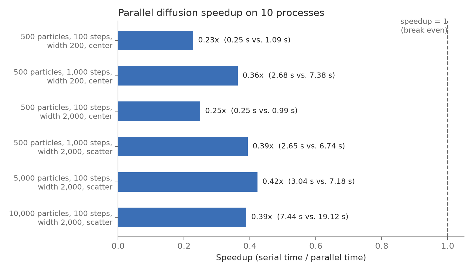
Running more steps helped a little, and so did scattering the particles. Scattering makes sense: when every particle starts in the center, the outer stripes have no particles at all, and their workers sit on the sidelines waiting for a particle to wander over. More particles helped too, but even with 10,000 particles, the parallel simulation was still well over twice as slow as the serial one.

Part of the problem is Python itself, which was not designed as a parallel programming language and carries more overhead per process than languages like Go, so that we must go farther out in the size of our data before we see an improvement. But the bigger issue is that our workers simply do not have enough to do. All each one does is take its stripe and push each point a tiny distance. To justify their creation, we would need both a lot of particles and a lot of steps, and a run like that would take minutes.

We could also reduce the overhead directly. Right now, we reassign every particle to a worker at every step, which means shipping every particle to a worker process and back at every step. If instead each worker kept its own particles and only occasionally received a new assignment, we would avoid most of that communication.

Looking ahead

We could chase a better speedup for plain diffusion, but we have a more interesting way to give our workers more to do. In the next code along, we will add chemical reactions to our particles, so that particles of different types can meet and react, like predators eating prey or a game of rock, paper, scissors played out by molecules. Every worker will then have to check for nearby particles as well as move them, which is exactly the kind of work that makes parallelism pay off.