Any Number of Processes and Timing the Speedup in Python

Code along video

Learning objectives

In the previous code along, we split the work of summing a list over exactly two processes. But your computer probably has many more cores than two, and the number of cores varies from machine to machine. In this code along, we will generalize our demo into a function sum_multi_procs() that divides the work of summing a list over any number of processes. We will then time this function against an ordinary serial sum, compute the speedup of the parallel approach, and confront the cost that every parallel program pays, called overhead.

Code along summary

Setup

We will continue working in python/src/parallel/main.py from the previous code along, which contains main(), sum_example_two_procs(), and partial_sum(). As a reminder, here is partial_sum(), which every one of our workers will run. It sums a slice of the data and places the result into a queue.

def partial_sum(data_slice: list[int], result_queue: multiprocessing.Queue) -> None:
    """
    Takes as input a list of integers and a queue and places the sum of the list's
    elements into the queue.
    Note that it doesn't return anything.
    """
    val = sum(data_slice)  # this is serial!
    # place the value into the queue
    result_queue.put(val)

From two workers to any number of workers

If we are splitting a task over a collection of worker bees, the most natural question to ask is how many bees we have. Then we can split the task into pieces of essentially equal size, one for each bee. Our two-process demo did this for two bees, but it would be much more elegant to write a function that works for any number of them.

Add the following function signature to main.py; we placed it above sum_example_two_procs(). Our function takes a list of integers data and an integer num_procs indicating the number of processes over which we will divide the work.

def sum_multi_procs(data: list[int], num_procs: int) -> int:
    """
    Divides work of summing an input list of integers over n processes.
    Returns the sum of all elements in the list.
    """

What is nice about this function is that from the outside, it looks like a normal old function: it takes a list of integers and returns an integer, its sum. The parallelism is hidden inside. And because num_procs is just a parameter, if Phillip’s computer has 10 cores and yours has 14, then he can split the work over 10 processes and you can split it over 14, each calling the same function with the value that is best for our own machine.

How big should each chunk be?

When we had two processes, dividing the data was easy: we split the list at its midpoint. Now we want to divide the input list into num_procs chunks of roughly equal size.

Each chunk should contain about len(data) // num_procs elements, where we use integer division because a chunk must contain a whole number of elements. But we need to be careful. Say that data has length 1003 and num_procs is equal to 10. Then the chunk size is 1003 // 10, which is 100 (with a remainder of 3). If every one of our 10 processes receives 100 elements, then together they handle only 1000 elements, and we will miss the last three.

The fix is to place the leftover elements in the final chunk. When we have a big data set, we will not have a huge number of processes, so the remainder (which is always smaller than num_procs) will only ever add a few extra elements to the last worker’s load. Add the following lines to sum_multi_procs().

# divide the input data list into num_procs equally sized chunks
chunk_size = len(data) // num_procs

# be careful: if len(data) = 1003, num_procs = 10, then chunk_size = 100
# we will put extra elements in the final process

Handling the leftover elements is the only part of this function that is harder than what we have already done. Everything else follows the same plan as before. We will create slices of our data of approximately equal size, define one process for each slice, start the processes, join them, and finally grab the values from the queue and add them together.

Slicing the data

We will first make a list data_slices whose elements are the sublists of data. Its type is a list of lists of integers, list[list[int]]. We do not need to include this type annotation (we could just write data_slices = []), but it is a good habit to think about what type each of our variables has.

We then range over our processes, using i to index them. Process i should start at index i * chunk_size and end at index (i + 1) * chunk_size. When the chunk size is 100, the first process receives indices 0 to 100, the second process receives indices 100 to 200, then 200 to 300, and so on. (As always with slicing, the end index is not included.) For the final process, when i is equal to num_procs - 1, we push the end index all the way to len(data) so that this process picks up the leftovers; in our running example, the final slice runs from index 900 to 1003.

# make a list containing my sublists
data_slices: list[list[int]] = []
for i in range(num_procs):
    start_index = i*chunk_size
    end_index = (i+1)*chunk_size
    # these indices will be [0, 100], [100, 200], [200, 300], etc.
    # be careful: last one should be [900, 1003]
    if i == num_procs - 1:
        end_index = len(data)

    current_list = data[start_index:end_index]
    data_slices.append(current_list)

Starting the workers

Now that we have split the data into pieces, we create our queue, which starts out empty. Every worker will place its partial sum into this queue.

result_queue = multiprocessing.Queue()  # this will store our results from each worker

Next, we need to start the work. With two workers, we could call p0.start() and p1.start(), but now we have num_procs workers, so we will store them in a list called processes whose elements have type multiprocessing.Process. We then range over the slices in data_slices (of which there are num_procs). For each slice, we declare a process p in exactly the same way as before: its target is the name of the function that we want it to call, partial_sum, and its args are the arguments for this function, given as a tuple. The only thing that differs from before is that the first argument is the current slice instead of data_slices[0]. We append each process to our list and start it, and then we join it.

# start the work!
processes: list[multiprocessing.Process] = []
for slice in data_slices:
    p = multiprocessing.Process(target=partial_sum, args = (slice, result_queue))
    processes.append(p)
    p.start()
    p.join()

We certainly want to call join() after start(), and we want to call it once for every process. The problem is where we call it. Recall that p.join() blocks, meaning that our code does not continue until p has finished.

Say that we have 10 processes. We start the first one and hand it one tenth of the data, and it begins working. Our code carries on to the next line, which is p.join(), so we sit and wait until the first process is completely finished. Only then do we return to the top of the loop, start the second process, and wait for it to finish. We have done all of the hard work of setting up our processes, but they run one at a time, so this code is no better than a serial program (and is actually worse, since we pay to create every process).

Instead, we must allow all of our processes to start, and only after they have all started should we join them. So we remove p.join() from the first loop and write a separate loop that joins the processes.

# start the work!
processes: list[multiprocessing.Process] = []
for slice in data_slices:
    p = multiprocessing.Process(target=partial_sum, args = (slice, result_queue))
    processes.append(p)
    p.start()

# after we have started all the processes, only then should we allow them to join
for p in processes:
    p.join()  # is k-th process finished? If yes, loop, if not, wait til it is

# high level: we only reach this point in the code if all processes are finished

The high-level way to think about this second loop is that we only reach the line after it once all of our processes are finished, and at that point, we have control back. If you would like to think at a lower level, the k-th time through the loop, we ask whether the k-th process is finished. If it is, we carry on and loop again; if not, we wait until it is. It does not matter if a later process finishes before an earlier one; when we reach a process that is already done, join() returns immediately.

If you write a lot of parallel code in this style, you will see this pattern over and over again: start the processes in one loop, then block for them in another.

Collecting the results

If all of our processes are finished, then all of their values are in the queue, and so we just need to get them. We declare a variable total_sum equal to zero and then range num_procs times, each time grabbing a value from the queue with get() and adding it to total_sum. We then return total_sum.

# this means all values are in the queue
total_sum = 0
for _ in range(num_procs):
    total_sum += result_queue.get()  # FIFO

return total_sum

Just as before, a queue is first in, first out (or FIFO, a term that anyone who has taken accounting may dread). The first process to finish puts its value into the queue first, and that value is the first one we take out. We are not forcing our processes to finish in any particular order; if we cared which value came from which worker, we would label the values, but here we only care about their sum.

Here is our completed function.

def sum_multi_procs(data: list[int], num_procs: int) -> int:
    """
    Divides work of summing an input list of integers over n processes.
    Returns the sum of all elements in the list.
    """
    # divide the input data list into num_procs equally sized chunks
    chunk_size = len(data) // num_procs

    # be careful: if len(data) = 1003, num_procs = 10, then chunk_size = 100
    # we will put extra elements in the final process

    # make a list containing my sublists
    data_slices: list[list[int]] = []
    for i in range(num_procs):
        start_index = i*chunk_size
        end_index = (i+1)*chunk_size
        # these indices will be [0, 100], [100, 200], [200, 300], etc.
        # be careful: last one should be [900, 1003]
        if i == num_procs - 1:
            end_index = len(data)

        current_list = data[start_index:end_index]
        data_slices.append(current_list)

    result_queue = multiprocessing.Queue()  # this will store our results from each worker

    # start the work!
    processes: list[multiprocessing.Process] = []
    for slice in data_slices:
        p = multiprocessing.Process(target=partial_sum, args = (slice, result_queue))
        processes.append(p)
        p.start()

    # after we have started all the processes, only then should we allow them to join
    for p in processes:
        p.join()  # is k-th process finished? If yes, loop, if not, wait til it is

    # high level: we only reach this point in the code if all processes are finished

    # this means all values are in the queue
    total_sum = 0
    for _ in range(num_procs):
        total_sum += result_queue.get()  # FIFO

    return total_sum

Look at this function from a distance, and you will notice that it hardly contains any parallelism. Dividing the data is serial. Creating the queue is serial. The work of the parallel processes happens in the two short loops in the middle, where we need to know a little about processes and blocking, and then collecting the results from the queue is serial again. This is good practice, in the same way that it is good practice to write modular code that calls many subroutines. At the highest level, we have a task that we divide over some number of processes; most of the code is ordinary serial code, and the parallel work is pushed to a subroutine (partial_sum()) that each worker runs.

Checking our function

Before going any further, let’s make sure that our function is correct. Add the following lines to main(), which sum the integers from 1 to 100 using eight processes.

def main():
    print("Parallel programming!")

    print("Num cores available:", multiprocessing.cpu_count())

    sum_example_two_procs()

    n = 100
    data = list(range(1, n+1))
    num_procs = 8
    print(sum_multi_procs(data, num_procs))

When we run python3 main.py, the last line printed is 5050, the same answer that Gauss found, so our function seems to be working.

Parallel programming!
Num cores available: 8
Sum of list elements is: 5050
5050

Phillip’s computer has 10 cores, and he divided the work into eight processes. He could have divided it into 16, and he would still get the right answer. Dividing the work into 10 pieces because we have 10 cores does not mean that Python will hand one piece to each core; we do not have control over the computer at that granular a level, and that is a good thing, because we don’t want that control. Still, if we have 10 cores, then it probably makes sense to divide the work into 10 pieces.

Both cases work. When the list has length 7 and we use 8 processes, the chunk size is 0, and so the first seven processes receive empty slices (whose sum is 0), while the final process receives all seven elements. Wasteful, but correct. We checked our function on lists of length 7, 10, 100, and 1003 using 1, 3, 8, 10, and 16 processes, and it returned the right sum every time.

Timing the serial and parallel approaches

Now that we have a parallel function for summing a list, what would we like to know about it? How long it takes, of course! To time our code, add an import of the time module to the top of main.py.

import multiprocessing
import time

Next, we will write a function timing_comparison() that times a serial approach for summing the elements of a list against our parallel approach. We start by creating a list containing the integers from 1 to n, where n is equal to 1000.

How many processes should we use? The number we have available. We can set num_procs equal to multiprocessing.cpu_count(), which makes our code very portable. We can hand this code to someone whose computer has 16 cores, or who has access to a supercomputer with 10,000 cores, or who is running an old computer with a single core, and in each case, num_procs will be set to the number of cores available on that machine. This is what is nice about having written sum_multi_procs() with the number of processes as a parameter.

def timing_comparison() -> None:
    """
    Times a serial approach for summing elements of a list against a parallel approach.
    """
    n = 1000
    data = list(range(1, n+1))

    # how many processes should I use? The number I have available
    num_procs = multiprocessing.cpu_count()

To time the parallel approach, we start a stopwatch by storing the current time from time.time() in a variable start_parallel. We then call sum_multi_procs(data, num_procs); we don’t care about its output, since we have already convinced ourselves that it is correct. Afterward, we stop the stopwatch by calling time.time() again and subtract the two values to obtain the time taken, in seconds.

We do the exact same thing for a serial approach. To make a fair, apples-to-apples comparison, we will use Python’s built-in sum() function, which is what each of our workers calls inside partial_sum(). (We know how to write this function ourselves: range over every element of the list and add it to a running total. At this point in the course, let’s take it for granted.)

start_parallel = time.time()
sum_multi_procs(data, num_procs)
end_parallel = time.time()
total_parallel = end_parallel - start_parallel
print("Time taken by parallel algorithm:", total_parallel)

start_serial = time.time()
sum(data)
end_serial = time.time()
total_serial = end_serial - start_serial
print("Time taken by serial algorithm:", total_serial)

Once we have both runtimes, there is always one more thing that we do, which is to ask how much faster the optimized algorithm is than the original one. This ratio is called the speedup, and we compute it by dividing the serial runtime by the parallel runtime. If the serial approach took a minute and the parallel approach took one second, then the speedup would be 60. Add the following line to the end of timing_comparison().

print(f"Speedup obtained by parallel approach: {total_serial/total_parallel}")

Finally, replace the test code in main() so that it calls timing_comparison(). We comment out the call to sum_example_two_procs() as well.

def main():
    print("Parallel programming!")

    print("Num cores available:", multiprocessing.cpu_count())

    # sum_example_two_procs()

    timing_comparison()

The disappointing results

In an ideal world, the speedup would be equal to the number of cores we have. With one core, we would obtain a speedup of 1; with two cores, a speedup of 2; on Phillip’s 10-core machine, a speedup of 10; and on a supercomputer with a thousand cores available, a speedup of 1000. That’s the dream. Here is what we obtain when we run python3 main.py on a laptop with 8 cores (your times will differ).

Parallel programming!
Num cores available: 8
Time taken by parallel algorithm: 1.499202013015747
Time taken by serial algorithm: 1.0013580322265625e-05
Speedup obtained by parallel approach: 6.679273530404769e-06

This output looks exciting until we look at the exponents. Our serial algorithm takes just a few millionths of a second, but our parallel algorithm takes over a second (this number jumps around a lot from run to run, depending on what else the computer is doing), so the parallel approach is many thousands of times slower. (In the video, the serial sum took about 4 × 10^-6 seconds, and the parallel sum took about 0.15 seconds.) This is a terrible speedup, so what can we do?

One thing that we can try is to increase the size of the data. Change n to 10,000, then 100,000, then a million, and so on, running the code each time. The time taken by the parallel algorithm grows only slowly at first, while the serial algorithm takes longer and longer, so the speedup starts to creep upward. In the video, the speedup rises from 0.0023 for a list of length 100,000 to 0.0072 for a million, then to 0.036 for ten million. For a list of length 100 million, the parallel algorithm took about 10 seconds and the serial algorithm took 1.73 seconds, for a speedup of about 0.17. Going much further than this, we run out of memory to store all of these integers.

The figure below shows the results when we ran this experiment ourselves, from 1000 up to 100 million elements.

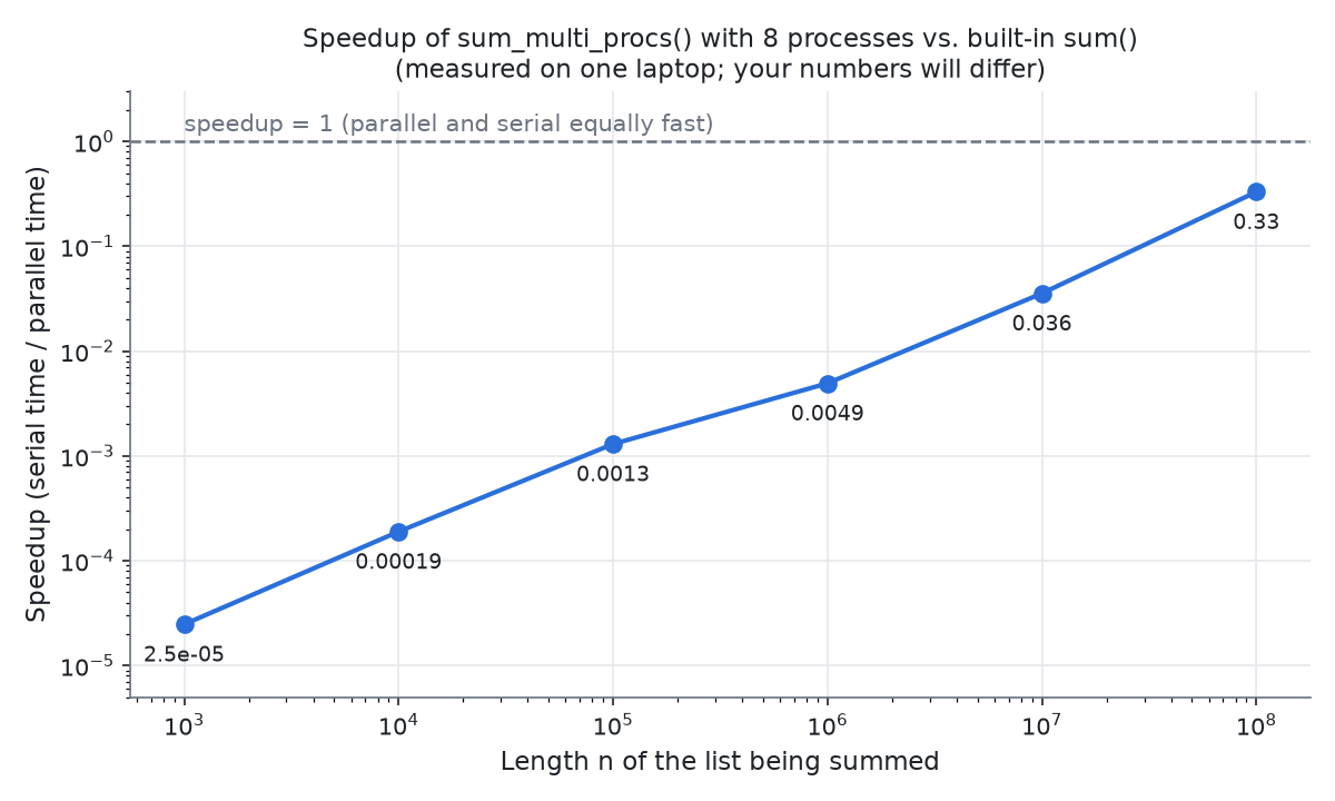
This picture is a vital mental image for how parallel programming works. As the size of our data grows, the speedup of a parallel algorithm compared to a serial algorithm often improves, which means that there is often a point at which the parallel algorithm becomes better. This is a subtler reason why we care about parallel algorithms in the first place. If you don’t have a lot of data, they may be pointless, but we are collecting more and more data all the time, and for large enough data sets, algorithms that run in parallel may win out.

In this example, though, we never reach that point. Fortunately, this means that we don’t need to call a parallel function every time we want to sum the elements of a list! The reason why is overhead.

Overhead

Phillip has moved from making students work on projects individually to allowing them to work in teams of up to four. He always tells them not to expect that working in a team of four means getting four times as much work done. A team needs coordination and communication among its members, and that costs time. In the same way, any parallel program pays an overhead, a fixed amount of time and resources that must be consumed to create and coordinate its workers. As a result, if we run a parallel algorithm on a computer with n cores, and we make a fair comparison against a serial algorithm, we should never expect the parallel algorithm to be n times faster. What we do expect is that the speedup will improve as the size of the data grows.

Our example suffers from overhead for two reasons. First, summing the elements of a list is trivial. Each worker spends almost no time on actual work, while creating a process and sending it a slice of the data is expensive. If each worker were doing something much more complicated, then the time saved by dividing the problem into 10 pieces could outweigh the overhead of introducing parallelism.

Second, Python gives us an unfair impression of how good parallel programming is. Python’s multiprocessing module carries a huge amount of overhead for setting up processes and organizing them, because parallel and distributed computing were bolted on to Python long after the language was introduced, instead of being designed into it from the ground up. Other languages have parallelism built in. When Phillip first taught this material roughly ten years ago, in what may have been the only introductory programming course in the world with parallel programming in it, he taught it in Go, a language that is great for tasks like running web servers precisely because parallel programming is part of the language. The demo in this lesson takes much less time to present in Go, and it needs much less navigation of overhead.

For these reasons, you are not likely to run a lot of parallel algorithms on a standard home laptop. But computing today happens at scale at least as much as on local machines: on supercomputers, on clusters, and on GPU setups with huge numbers of cores. And as we will see, Python’s support for parallelism will still let us do some really cool things, provided that we give our workers enough work to do.

Looking ahead

We now have a reusable pattern for parallel programs: divide the work into one piece per process, start every process in one loop, join them in another, and collect the results from a queue. But summing a list gave our workers too little to do. In the next code along, we will apply this pattern to a problem with much more work per worker, Monte Carlo simulation of the dice game craps, which is a very natural problem to parallelize. Later in the chapter, we will divide a two-dimensional space into strips and hand one strip to each process, which will let us simulate reaction-diffusion systems.