Parallel Reaction-Diffusion: Processing Strips in Python

Code along video

Learning objectives

In the previous code along, we wrote simulate_parallel(), which hands each worker a strip of the board along with that strip’s halo. In this code along, we will write the function that every worker runs, process_strip(), which moves the particles in a strip and its halo and then applies reactions, using the halo particles as catalysts that can change the strip’s particles but are never changed themselves. We will then finish simulate_parallel() by handling the steps left over at the end of the simulation, run our serial and parallel simulators side by side, and time the speedup. Along the way, we will see that giving our workers enough to do makes all the difference, and we will even see a speedup larger than the number of cores on the machine.

Code along summary

Setup

We will continue working in parallel.py within the reaction_diffusion directory from the previous code along (if you are starting fresh, download reaction-diffusion-python.zip here and complete the previous three code alongs first).

Telling a worker whether to react

When simulate_parallel() calls pool.starmap(), each worker runs process_strip() on its own tuple of arguments. The starter code gives this function six parameters: the particles in the worker’s strip, the particles in its halo, the reaction table, the simulation parameters, the number of steps to run (steps_to_run), and a boolean called do_reactions.

We need do_reactions because of the remainder. Recall that we apply reactions once per batch of params.proximity_interval steps, and if params.num_steps is not divisible by params.proximity_interval, then a few steps are left over at the end. During those leftover steps, particles should move according to their random walks, but they should not react, since the steps do not make a full batch. So in every full batch, a worker should apply reactions, which means that the tuple that we build for each worker in the loop over batches needs one more element, True.

# next, create list of all the arguments that are passed as inputs to each worker
worker_args: list[tuple] = []
for i in range(num_procs):
    worker_args.append((strips[i], halos[i], table, params, params.proximity_interval, True))

Running the leftover steps

Next, after the loop over batches (and before we fire the workers), we handle this minor, annoying case of the leftover steps, which only arise if remainder is greater than zero. The work is nearly identical to a single batch. We assign the particles to strips with halos, build a new list of worker arguments, call starmap(), and compile the results into a new snapshot. The only differences are that each worker runs remainder steps instead of params.proximity_interval, and that its final argument is False, so that it moves its particles without applying reactions.

# run any leftover steps that are remaining that don't involve reactions
if remainder > 0:
    strips, halos = assign_strips_with_halos(current, num_procs, params.width, params.activation_range)

    worker_args = []
    # range over all workers and give each one what it needs
    for i in range(num_procs):
        worker_args.append((strips[i], halos[i], table, params, remainder, False))

    results = pool.starmap(process_strip, worker_args)

    # now we compile the results, list[list[Particle]]
    current = []
    for strip in results:  # strip is list[Particle]
        current.extend(strip)

    # now, current is set: all particles in our snapshot
    frames.append(current)

Whenever we copy this much code, the subroutine sirens should be going off in our heads. Phillip does not see a natural way to place this code in a subroutine, since it differs from a batch only in the number of steps and the True/False flag, but it is worth trying.

Here is our finished simulate_parallel().

def simulate_parallel(particles: list[Particle],
                      table: ReactionTable,
                      params: SimulationParameters,
                      num_procs: int) -> list[list[Particle]]:
    # first, let's make the current list of particles and the list of "snapshots" that we eventually want to return
    current: list[Particle] = copy.deepcopy(particles)
    frames: list[list[Particle]] = [copy.deepcopy(current)]

    # question: how many snapshots will I eventually take?
    # remember: proximity_interval = number of steps between snapshots
    num_batches = params.num_steps // params.proximity_interval
    remainder = params.num_steps % params.proximity_interval

    # let's make our worker pool
    pool = multiprocessing.Pool(num_procs)

    # again, we divide into batches
    for _ in range(num_batches):
        # divide the space into vertical strips
        # key tricky point: each worker needs to know the collection of points that fall in its strip + the collection of particles that are close enough to its strip to maybe be involved in a reaction
        strips, halos = assign_strips_with_halos(current, num_procs, params.width, params.activation_range)

        # next, create list of all the arguments that are passed as inputs to each worker
        worker_args: list[tuple] = []
        for i in range(num_procs):
            worker_args.append((strips[i], halos[i], table, params, params.proximity_interval, True))

        # now we call the critical pool method (starmap)
        # this is where the parallelization happens
        results = pool.starmap(process_strip, worker_args)

        # now we compile the results, list[list[Particle]]
        current = []
        for strip in results:  # strip is list[Particle]
            current.extend(strip)

        # now, current is set: all particles in our snapshot
        frames.append(current)

    # run any leftover steps that are remaining that don't involve reactions
    if remainder > 0:
        strips, halos = assign_strips_with_halos(current, num_procs, params.width, params.activation_range)

        worker_args = []
        # range over all workers and give each one what it needs
        for i in range(num_procs):
            worker_args.append((strips[i], halos[i], table, params, remainder, False))

        results = pool.starmap(process_strip, worker_args)

        # now we compile the results, list[list[Particle]]
        current = []
        for strip in results:  # strip is list[Particle]
            current.extend(strip)

        # now, current is set: all particles in our snapshot
        frames.append(current)

    # at the end of the process, fire all the workers
    pool.close()
    pool.join()

    return frames

Writing process_strip()

We now zoom in on a single worker, which is in charge of one strip along with its halo. This function is not too bad, because it is our serial algorithm in miniature. First, we move every particle in the strip and the halo steps_to_run times by calling the rand_step() function that we already wrote in functions.py, passing it the width and height of the board from params.

def process_strip(strip_particles: list[Particle],
                  halo_particles:  list[Particle],
                  table:           ReactionTable,
                  params:          SimulationParameters,
                  steps_to_run:    int,
                  do_reactions:    bool) -> list[Particle]:
    # first, move all the particles in the strip and the halo the appropriate number of steps
    for _ in range(steps_to_run):
        for p in strip_particles:
            rand_step(p, params.width, params.height)
        for p in halo_particles:
            rand_step(p, params.width, params.height)

Our strip’s particles have moved for steps_to_run steps, and if the halo particles stood still, then the particles in the strip would react with neighbors that are frozen in time. Moving the halo keeps each halo particle’s position a plausible one for the end of the batch. The copy of a halo particle on our worker will not be in exactly the same place as the copy on the worker that owns it, since the two take different random steps. But because a random walk is random, both positions are equally valid outcomes, and the only position that persists is the one returned by the owner. The halo particles are like visitors from across the border: they can influence what happens in our strip, but they report back to someone else.

Next, if do_reactions is True, we apply the reactions. We pass the work for contact reactions to a subroutine, apply_reactions_with_halo(), which needs the strip particles, the halo particles, the table, and the parameters. Then we update the strip particles one more time by applying unary reactions with the apply_unary_reactions() function that we wrote in functions.py, which is already imported at the top of parallel.py. Fortunately, unary reactions do not involve a halo, since a particle that is born, dies, or changes from one species to another on its own does not need to look across the fence at a partner in another strip. All of this can happen within the boundaries of the strip that this worker owns. Finally, we return the strip’s particles.

def process_strip(strip_particles: list[Particle],
                  halo_particles:  list[Particle],
                  table:           ReactionTable,
                  params:          SimulationParameters,
                  steps_to_run:    int,
                  do_reactions:    bool) -> list[Particle]:
    # first, move all the particles in the strip and the halo the appropriate number of steps
    for _ in range(steps_to_run):
        for p in strip_particles:
            rand_step(p, params.width, params.height)
        for p in halo_particles:
            rand_step(p, params.width, params.height)

    # second part is to apply the reactions
    if do_reactions:
        strip_particles = apply_reactions_with_halo(strip_particles, halo_particles, table, params)
        # fortunately, unary reactions don't involve a halo
        strip_particles = apply_unary_reactions(strip_particles, table, params)

    return strip_particles

Applying reactions with a halo

It remains to implement apply_reactions_with_halo(), which takes the particles in the worker’s strip, the particles near enough to the strip to be possible reaction partners, the reaction table, and the simulation parameters. It returns the list of strip particles after reactions are applied. We have already done nearly all of this work in apply_reactions() in functions.py, so we can almost copy that function over.

The only difference is the halo. A substrate (the particle that may change) must come from the strip, since this worker only owns the strip’s particles. But a catalyst (the particle that causes the change) can be either in the strip or in the halo. So we form a list catalysts that is the concatenation of strip and halo, and then we range over every substrate in the strip and every catalyst in catalysts. The rest of the function is the same as before: skip a particle paired with itself, check the reaction table first because it is the quicker test, then check whether the two particles are within the activation range on our torus, and if so, roll the dice. If the reaction fires, we update the substrate’s species to the reaction’s product, which is just an integer.

def apply_reactions_with_halo(strip: list[Particle],
                              halo:  list[Particle],
                              table: ReactionTable,
                              params: SimulationParameters) -> list[Particle]:
    # possible catalysts are both the strip itself and the halo
    catalysts = strip + halo

    # range over all the possible pairs and see if there's a reaction
    for substrate in strip:
        for catalyst in catalysts:
            if catalyst is not substrate:  # don't have reaction with yourself
                # two things: is there a reaction involving these two?
                # are they close enough (within threshold distance) to actually react?
                # first test is faster, so we want to do it first
                reaction = table.table[catalyst.species][substrate.species]
                if reaction is not None:
                    # now we know that there is a reaction involving them
                    # now we check to see if they're close
                    d = toroidal_distance(catalyst.position, substrate.position, params.width, params.height)
                    if d <= params.activation_range:
                        # both are true, then we roll some dice to see if we apply the reaction to these particles
                        if random.random() < reaction.rate:
                            # update substrate to whatever the reaction gives
                            substrate.species = reaction.product

    return strip

As with apply_reactions(), the strip list is mutated in place, and we return it for convenience.

If a halo particle’s species changed on our worker, then that change would be lost, since we never return the halo. Worse, the particle is a substrate on the worker that owns it, so if we let halo particles change as well, a single particle would get two chances to react with the same neighbors. Treating the halo as read-only means that each particle is tested as a substrate exactly once per batch, by the one worker that owns it, just as in our serial simulation.

Running the simulation

We are at mile 25 of our marathon. What we care about now is that the simulation runs, that it produces sensible results, and that it gives us a comparison of the serial and parallel algorithms. The main.py file that came with the starter code takes care of all of this. It runs simulate_serial() and then simulate_parallel() on the same initial particles, using as many processes as the computer has cores, renders an animation and a plot of species counts for each one in output, and prints the time that each simulation took. We run it from the reaction_diffusion directory with a command of the following form.

python3 main.py random data/reactions_gray_scott.csv 50 200 200 100

The first argument is either random, which scatters all the particles across the board, or clustered, which places each species in its own vertical stripe. The second argument is a CSV file of reactions; the data folder contains many examples. The third is the number of particles of each species, so that with three species and a value of 50, we will have 150 particles in total. The last three arguments are the width and height of the board and the number of steps to run.

We will use the Gray-Scott reactions in data/reactions_gray_scott.csv. If you completed the practice exercises accompanying our work on cellular automata, then this is essentially the same system that you simulated there, except that instead of zooming way out and viewing the system as an automaton, we zoom way in and watch individual particles interact. Here are the lines of the file after its explanatory comments.

diffusion,0,4
diffusion,1,1
diffusion,2,4
name,0,U
name,1,V
name,2,P
color,0,76,155,232
color,1,232,196,76
color,2,40,40,60
background,18,18,31
1,0,1,0.5
spontaneous,1,2,0.04
spontaneous,2,0,0.06

Each of the three species, which are called U, V, and P, has a diffusion rate, a color, and a name, and the board has a background color. The line 1,0,1,0.5 says that when a particle of species 1 (V) is within the activation range of a particle of species 0 (U), the U particle becomes a V particle with probability 0.5; you can think of V as a predator eating its prey and reproducing. The next two lines are spontaneous reactions: a V particle turns into species 2 (P) with probability 0.04, and a P particle turns into a U particle with probability 0.06. Species 2 is a trick that lets us simulate deaths and births without changing the number of particles: predators die by turning into P, and new prey are born from P. What we really care about are species 0 and 1.

When Phillip runs the command above, his first attempt crashes with the following error.

  File "/Users/phillipcompeau/python/src/reaction_diffusion/parallel.py", line 78, in simulate_parallel
    worker_args.append(strips[i], halos[i], table, params, params.proximity_interval, True)
    ~~~~~~~~~~~~~~~~~~^^^^^^^^^^^^^^^^^^^^^^^^^^^^^^^^^^^^^^^^^^^^^^^^^^^^^^^^^^^^^^^^^^^^^^^
TypeError: list.append() takes exactly one argument (6 given)

The append() method takes exactly one argument, but in the video Phillip has called it with six, because he left out the parentheses that bundle the six values into one tuple. Our code above already has these parentheses, so you should not see this error. After adding them (in both loops), the simulation runs. Here is the output from running the command on an eight-core laptop; your times will differ.

Reaction-diffusion simulation!
Loaded 3 species and 150 particles.
Output: output/gray_scott/
Running serial simulation.
Serial simulation complete in 0.431s.
Rendering serial animation.
  Animation written to output/gray_scott/serial.mp4  (21 frames @ 30 fps)
  Species count plot saved to output/gray_scott/serial_counts.png
Running parallel simulation (8 processes).
Parallel simulation complete in 0.781s.
Rendering parallel animation.
  Animation written to output/gray_scott/parallel.mp4  (21 frames @ 30 fps)
  Species count plot saved to output/gray_scott/parallel_counts.png

--- Timing ---
Serial:   0.431s
Parallel: 0.781s (8 processes)
Speedup:  0.55x
Animation finished! Exiting normally.

When you open output/gray_scott/serial.mp4 and output/gray_scott/parallel.mp4, the animations will look ugly, since we used a tiny 200 × 200 board, but the particles are moving and their species are changing. The species counts in serial_counts.png and parallel_counts.png will not be identical, since the simulation is random, but they should follow the same trends: with these reactions, the number of U particles drops quickly as the V particles consume them.

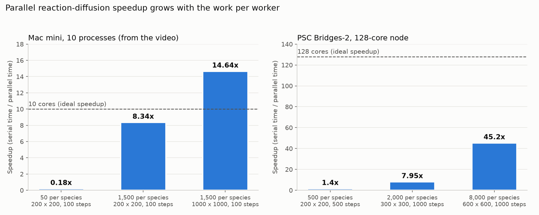
And yet, alas, the serial algorithm is faster than the parallel one. Phillip’s ten-core computer obtained a speedup of 0.18x in the video (serial: 0.040 seconds, parallel: 0.219 seconds). With only 150 particles, each worker has hardly any work to do, and the time spent creating the workers and copying particles back and forth with each batch dominates the running time.

Keeping the workers busy

Our workers have something sophisticated to do, since they apply all of these chemical reactions, but to keep them busy, we need to give them enough particles. When Phillip changes the number of particles per species from 50 to 1,500 and leaves everything else the same, the serial simulation takes 17.533 seconds, and the parallel simulation takes 2.102 seconds, an 8.34x speedup.

python3 main.py random data/reactions_gray_scott.csv 1500 200 200 100

Next, he keeps 1,500 particles per species but enlarges the board to 1000 × 1000. The serial simulation takes about the same time as before, 18.006 seconds, but the parallel simulation now takes only 1.230 seconds, for a speedup of 14.64x.

python3 main.py random data/reactions_gray_scott.csv 1500 1000 1000 100

Our serial simulator compares every particle against every other particle, so with n particles, it considers about n² pairs per batch. With p workers, each worker owns about n/p particles and compares them only against the particles in its strip and halo. If the halo were empty, each worker would consider about (n/p)² pairs, so that all p workers together would consider only n²/p pairs. In other words, by dividing the board into strips, we have not only split the work among the workers; we have also eliminated most of the work, since a particle never checks the distance to a particle on the far side of the board. This is why the parallel simulator can be more than p times faster than the serial one.

The halo is what keeps this from being even better. On a 200 × 200 board with 10 strips, each strip is 20 units wide, but the halo extends 28 units (the activation range) on each side, so each worker compares its particles against two entire neighboring strips. On a 1000 × 1000 board, each strip is 100 units wide, and the halo is a much smaller fraction of the work. This explains why enlarging the board improved the speedup from 8.34x to 14.64x even though the serial time hardly changed.

Phillip also ran this simulator on a single 128-core node of the Bridges-2 supercomputer at the Pittsburgh Supercomputing Center, using larger simulations. The speedup grows from 1.4x on a small run to 45.2x on a run with 8,000 particles of each of two species on a 600 × 600 board for 1,000 steps, which took 441.9 seconds in serial and 9.8 seconds in parallel. The figure below summarizes these measurements.

Unfortunately, at these sizes, we will not see the Turing patterns that the Gray-Scott reactions produce in a cellular automaton. These stripes and spots only emerge when we run the simulation with an enormous number of particles and step way back from the picture. In Phillip’s Biological Modeling course, he and his colleagues ran a particle simulation like this one for about eight hours to produce a short video in which Turing patterns emerge. Because a cellular automaton gives us these patterns much more cheaply, the Gray-Scott system is not the most interesting one for our particle simulator.

Looking ahead

Our parallel reaction-diffusion simulator is complete, and it produces the same kind of results as our serial simulator, only much faster when the workers have enough to do. In the next lesson, we will put it to use, taking a tour of reaction systems that a particle simulator brings to life, starting with a classic predator-prey model.