Code along video
Learning objectives
In the previous code along, we wrote the engine of our serial reaction-diffusion simulator and taught each particle to take a random step. Now we will make the particles react. We will write apply_reactions(), which handles contact reactions between pairs of nearby particles, and apply_unary_reactions(), which handles the reactions involving a single particle: death, spontaneous conversion, and birth. Along the way, we will see why the order of two tests can matter a great deal for speed, and we will compute distances on a board whose edges wrap around. By the end, our serial simulator will be complete, and we will run it.
Code along summary
Setup
We will continue working in the reaction_diffusion directory from the previous code along, filling in the three remaining functions in functions.py.
Applying contact reactions
Recall that simulate_serial() calls apply_reactions() once per batch of steps. This function takes three inputs: the list of particles, the reaction table describing every reaction that could happen (there could be a huge number of them, although our examples will have only a few), and the parameters of the simulation, such as the width and height of the board and the threshold distance within which two particles can react.
A contact reaction only changes the species of a particle; no particles are created or destroyed. So we could modify the list of particles in place and return nothing. Instead, much as we did back when we worked with cellular automata, we will return the list at the end, which allows simulate_serial() to use the same pattern, current = apply_reactions(current, table, params), for both kinds of reactions.
def apply_reactions(particles: list[Particle],
                    table: ReactionTable,
                    params: SimulationParameters) -> list[Particle]:
    # apply contact reactions

    return particles
We will make one simplifying assumption: every contact reaction involves exactly two particles. Three particles of different species could collide in the same place and react, but such events are much rarer than collisions of two particles, and most simulations ignore them (and nearly all simulations ignore four-particle collisions, which are astronomically rarer still).
To find all pairs of particles that might interact, we range over the list of particles twice. The outer particle is the substrate, the particle that might change. The inner particle is the catalyst, the particle that stays the same. For example, in the reaction A + B → A + C, the catalyst is the A particle, and the substrate is the B particle, which becomes a C.
We should not let a particle react with itself, which we check with the keyword is not. This test asks whether the two variables refer to literally the same object; it does not ask whether the two particles have the same species. Two predators can certainly meet and react, but a particle should not react with itself. (Maybe that is good advice to live by in general.)
# find all pairs of particles that might interact
# range over list twice
for substrate in particles:
    for catalyst in particles:
        if catalyst is not substrate:  # don't have reaction with yourself
            # two things: is there a reaction involving these two?
            # are they close enough (within threshold distance) to actually react?
Once we have a pair of distinct particles, two things must be true for a reaction to happen. First, the reaction table must contain a reaction involving the two particles’ species. Second, the particles must be within the threshold distance of each other. If both are true, then we roll the dice to see if the reaction occurs, since each reaction has a rate that serves as its probability.
STOP: Does it matter which of these two conditions we test first? If so, which one should we test first, and why?
We certainly should not roll the dice until we know that both conditions hold. But the order of the two tests matters too. As a general rule, when we need two conditions to both be true, we should test the one that is computationally cheaper first, since if it fails, we can skip the expensive test entirely.
Which test is cheaper? Checking whether a reaction exists requires a single lookup in a two-dimensional list. Checking whether two particles are close requires applying the distance formula, with its squares and square root. That may not seem like much more work, but as our simulation scales to tens or hundreds of thousands of particles over a huge number of steps, it adds up. Furthermore, on a large board with a small threshold distance, most pairs of particles will be far apart, so if we computed the distance first, we would spend most of our time computing distances that tell us nothing. The table lookup instead winnows down the pairs, so that we only compute distances for a much smaller subset.
Recall that the ReactionTable type has a table attribute, which is a two-dimensional list of ContactReaction objects (or None when two species do not react). Because species are represented as integers, we access the reaction in which catalyst acts on substrate as table.table[catalyst.species][substrate.species]. If this value is not None, then we know that a reaction involving the two particles exists.
Only then do we compute the distance d between the two particles. This distance comes with a twist. Our board is a torus, so a particle near an edge may be close to particles that are on the other side of the board, and a particle near a corner may be close to particles in any of the four corners. We will therefore delegate this computation to a function called toroidal_distance(), which we will write shortly. This extra work makes the distance test even slower compared to the table lookup.
If d is within the threshold distance, which is stored as the activation_range attribute of params, then we come to the small piece of our algorithm that is Monte Carlo. We generate a random decimal between 0 and 1 with random.random(); if it is smaller than the reaction’s rate, then the reaction happens, and we update the substrate’s species to the reaction’s product. For example, when a predator (the catalyst) meets a prey (the substrate), the prey becomes a predator.
def apply_reactions(particles: list[Particle],
                    table: ReactionTable,
                    params: SimulationParameters) -> list[Particle]:
    """Apply contact reactions: pair every particle with every other particle.

    For each ordered pair of distinct particles (A, B), we ask the reaction
    table what happens if A meets B. If table.table[A.species][B.species] is
    a ContactReaction and the pair is within activation_range (toroidally),
    B's species is changed to the reaction's product with probability
    reaction.rate. A is the "catalyst" (unchanged); B is the "substrate"
    (the one that may change).

    In each iteration of the outer loop, the same particle plays the
    substrate role; in the inner loop it plays the catalyst role for every
    other particle. So every particle is potentially both -- this is what
    "ordered pairs" means here.

    The list is mutated in place (only the species attribute changes; no
    particles are added or removed). We also return the list so the caller
    can use the same `current = apply_reactions(...)` pattern as
    apply_unary_reactions.

    Args:
        particles: Every particle in the simulation. Modified in place.
        table:     ReactionTable for conversion lookups.
        params:    Simulation parameters.

    Returns:
        The particles list (the same object as the input).
    """
    # find all pairs of particles that might interact
    # range over list twice
    for substrate in particles:
        for catalyst in particles:
            if catalyst is not substrate:  # don't have reaction with yourself
                # two things: is there a reaction involving these two?
                # are they close enough (within threshold distance) to actually react?
                # first test is faster, so we want to do it first
                reaction = table.table[catalyst.species][substrate.species]
                if reaction is not None:
                    # now we know that there is a reaction involving them
                    # now we check to see if they're close
                    d = toroidal_distance(catalyst.position, substrate.position)
                    if d <= params.activation_range:
                        # both are true, then we roll some dice to see if we apply the reaction to these particles
                        if random.random() < reaction.rate:
                            # update substrate to whatever the reaction gives
                            substrate.species = reaction.product

    return particles
That is a lot of nesting: two for loops and three if statements. We could flatten the inner tests by combining them with and, but the resulting line would be hideous, and the temporary variables reaction and d make the logic easier to read while costing us nothing. Sometimes nesting is OK.
Note: Keep an eye on the call totoroidal_distance()in this function. We will need to come back to it after we writetoroidal_distance().
Applying unary reactions
Next, we turn to apply_unary_reactions(), which handles reactions that do not require contact. We are lumping three types of reaction together here: a particle can die, a particle can spontaneously convert from one species to another, and a particle can give birth to a new particle. We will handle the three types one after another; you could rearrange their order, which would change the simulation only very slightly.
This function takes the same inputs as apply_reactions(), but this time, we will build and return a new list of particles, since some particles will die and others will be born. We make two empty lists, survivors and births, and at the end, we return their concatenation with +, which we have seen is a quick and convenient way to combine two lists in Python.
def apply_unary_reactions(particles: list[Particle],
                          table: ReactionTable,
                          params: SimulationParameters) -> list[Particle]:
    """Apply spontaneous (contact-free) reactions: deaths, conversions, births.

    For each particle:
      1. Roll the death rule for its species (if any). A dead particle
         won't make it into the survivor list.
      2. If still alive, roll the spontaneous-conversion rule for its
         species (if any). The species attribute may be overwritten.
      3. Roll the birth rule for its species (if any). Birth is independent
         of death -- a particle dying this batch can still leave behind one
         offspring before being removed.

    Args:
        particles: Particle list (read-only here; we return a fresh list).
        table:     ReactionTable defining unary, birth, and death rules.
        params:    Simulation parameters (provides box size).

    Returns:
        A new particle list containing the survivors plus any newly born
        particles. The caller should reassign their reference.
    """
    # create two lists that will be useful: one for survivors, one for births
    survivors: list[Particle] = []
    births: list[Particle] = []

    # apply each of the three reaction types

    return survivors + births
For each particle, we first ask whether it dies. We set a Boolean variable dead to False and then range over the table’s death_reactions attribute, a list of DeathReaction objects. Each death reaction has a species attribute and a rate attribute. Not every species can die; if we have ten species, eight of them might be immortal. So we check whether the particle’s species matches the death reaction’s species, and if it does, we roll the dice; if random.random() is smaller than the death reaction’s rate, we set dead to True.
Second, we ask whether the particle changes species, which only makes sense if the particle is still alive. We range over the table’s unary_reactions attribute, a list of UnaryReaction objects, each of which has a from_species attribute, a to_species attribute, and a rate. If the particle’s species matches from_species, then we roll the dice once more, and if we win, the particle’s species becomes to_species.
for particle in particles:
    # rule #1: does it die out?
    dead = False
    for d in table.death_reactions:
        if particle.species == d.species:
            # we find that this particle can die
            # does it?
            if random.random() < d.rate:
                dead = True

    # now we'll move on to rule 2: does it change?
    # it can only change from one species to another if it's alive
    if not dead:
        for u in table.unary_reactions:
            if particle.species == u.from_species:
                if random.random() < u.rate:
                    particle.species = u.to_species
Third, we ask whether the particle gives birth. Birth reactions are stored in the table’s birth_reactions attribute; like death reactions, each one has a species and a rate. If the particle’s species matches and we win one more roll of the dice, then we create a new particle and append it to births.
The new particle has the same species, radius, and diffusion rate as its parent, but where should we put it? We will place it at a random position on the board, choosing its x-coordinate uniformly between 0 and the width of the board with random.uniform(), and its y-coordinate uniformly between 0 and the height.
Finally, if the particle survived rule 1, we append it to survivors. Here is the finished function.
def apply_unary_reactions(particles: list[Particle],
                          table: ReactionTable,
                          params: SimulationParameters) -> list[Particle]:
    """Apply spontaneous (contact-free) reactions: deaths, conversions, births.

    For each particle:
      1. Roll the death rule for its species (if any). A dead particle
         won't make it into the survivor list.
      2. If still alive, roll the spontaneous-conversion rule for its
         species (if any). The species attribute may be overwritten.
      3. Roll the birth rule for its species (if any). Birth is independent
         of death -- a particle dying this batch can still leave behind one
         offspring before being removed.

    Args:
        particles: Particle list (read-only here; we return a fresh list).
        table:     ReactionTable defining unary, birth, and death rules.
        params:    Simulation parameters (provides box size).

    Returns:
        A new particle list containing the survivors plus any newly born
        particles. The caller should reassign their reference.
    """
    # create two lists that will be useful: one for survivors, one for births
    survivors: list[Particle] = []
    births: list[Particle] = []

    # apply each of the three reaction types

    for particle in particles:
        # rule #1: does it die out?
        dead = False
        for d in table.death_reactions:
            if particle.species == d.species:
                # we find that this particle can die
                # does it?
                if random.random() < d.rate:
                    dead = True

        # now we'll move on to rule 2: does it change?
        # it can only change from one species to another if it's alive
        if not dead:
            for u in table.unary_reactions:
                if particle.species == u.from_species:
                    if random.random() < u.rate:
                        particle.species = u.to_species

        # rule 3: is there a new particle born?
        for b in table.birth_reactions:
            if particle.species == b.species:
                # roll the dice one more time,
                if random.random() < b.rate:
                    # if there's a win, place it randomly
                    births.append(Particle(position = OrderedPair(
                                           x = random.uniform(0.0, params.width),
                                           y = random.uniform(0.0, params.height)),
                                           species = particle.species,
                                           radius = particle.radius,
                                           diffusion_rate=particle.diffusion_rate))

        # at this point in time, if the particle has survived all this, then we want it to add it to the survivors
        if not dead:
            survivors.append(particle)

    return survivors + births
The Particle(...) call is spread over several lines so that its arguments line up, which is about as pretty as we can make it.
STOP: As written, a particle that dies in rule 1 can still give birth in rule 3. Is that a problem? How could you change one line to prevent it?
We could prevent dead particles from giving birth by adding and not dead to the birth test. But this is a modeling choice more than a bug: you could imagine a particle reproducing just before it dies, or performing these three rules in a different order. Either way, the change has little effect on the simulation, and the docstring tells us that this behavior is intended.
Toroidal distance
We have one function left, toroidal_distance(), which takes two positions p0 and p1 along with the width and height of the board. If we ignore the torus for a moment, we just need the distance formula: we compute the absolute differences dx and dy between the x- and y-coordinates, and we return the square root of dx*dx + dy*dy.
dx = abs(p0.x-p1.x)
dy = abs(p0.y-p1.y)

return math.sqrt(dx*dx + dy*dy)
The trick is to account for the torus without changing this code much. Say that the width of the board is 1000, p0.x is 1, and p1.x is 999. Then dx is 998, but if we wrap around the edge of the board, the two points are only 2 units apart in the x direction. In general, wrapping around gives a distance of width-dx in the x direction, and similarly height-dy in the y direction. So we update dx to be the smaller of dx and width-dx, and we update dy in the same way. We could do this with the built-in min() function, but we will use if statements.
dx = abs(p0.x-p1.x)
dy = abs(p0.y-p1.y)

# trick: we "wrap around" if when wrapping around, distance in the x direction is smaller than dx (or the same for dy)
# width = 1000, p0.x = 1, p1.x = 999 -- dx = 998, but they're actually 2 away
# idea: update dx, and dy to be min of their current values and width-dx or width-dy
if width-dx < dx:
    dx=width-dx
if width-dy < dy:
    dy=height-dy

return math.sqrt(dx*dx + dy*dy)
STOP: There is a subtle bug in this code that will not show up if the board is square. Can you find it?
The test for dy compares against width-dy instead of height-dy. On a square board, the width and height are equal, so no harm is done. But consider our 800 × 600 board and two particles whose y-coordinates differ by 350, so that dy is 350. Wrapping around, they are only 600 – 350 = 250 apart in the y direction. However, the code checks whether 800 – 350 = 450 is less than 350, which is false, so it keeps the larger value of 350, and the two particles may wrongly be judged too far apart to react. Here is the corrected function.
def toroidal_distance(p0: OrderedPair, p1: OrderedPair,
                      width: float, height: float) -> float:
    """Shortest distance between two points on a periodic (torus) box.

    A particle at x=0 and a particle at x=width-1 are 1.0 apart on the torus,
    not width-1 apart. This matches the wrap-around motion done by
    rand_step.

    Args:
        p0:     First point.
        p1:     Second point.
        width:  Box width (the periodic length along x).
        height: Box height (the periodic length along y).

    Returns:
        Shortest periodic distance as a float.
    """
    dx = abs(p0.x-p1.x)
    dy = abs(p0.y-p1.y)

    # trick: we "wrap around" if when wrapping around, distance in the x direction is smaller than dx (or the same for dy)
    # width = 1000, p0.x = 1, p1.x = 999 -- dx = 998, but they're actually 2 away
    # idea: update dx, and dy to be min of their current values and width-dx or height-dy
    if width-dx < dx:
        dx=width-dx
    if height-dy < dy:
        dy=height-dy

    return math.sqrt(dx*dx + dy*dy)
Note: In the video, the y test is typed asif width-dy < dy:. We have corrected it toif height-dy < dy:above. The bug only matters when the board is not square, but sincemain.pylets us choose any width and height, make sure that your code usesheight.
Now let’s return to the call that we flagged in apply_reactions(). Our function has four parameters, but in the video, apply_reactions() passes it only the two positions. If we ran the simulation as is, Python would raise a TypeError complaining that toroidal_distance() is missing the arguments width and height. We need to pass the width and height of the board from params, so we update that line as follows.
d = toroidal_distance(catalyst.position, substrate.position, params.width, params.height)
Note: Phillip catches this missing-argument bug later in the stream, when he writes the same call in the parallel version of the reaction step. We fix it here so that the serial simulator runs.
Trying out the serial simulator
Our serial simulator is now complete! The main.py provided with the starter code runs both the serial simulator and the parallel simulator and compares them, so we cannot use it until we write the parallel version in the coming code alongs. In the meantime, if you would like to see your serial simulator in action, create a small file called run_serial.py in the reaction_diffusion directory. It loads the Lotka-Volterra predator-prey reactions from the data folder, scatters 50 prey and 50 predators randomly over an 800 × 600 board, runs 1000 steps (200 batches of 5 steps each), and prints the number of each species every 25 frames.
"""
run_serial.py

A quick test of the serial reaction-diffusion simulator, before we write
the parallel version.
"""

import time

from custom_io import load_reaction_table, make_random_particles
from datatypes import Particle, ReactionTable, SimulationParameters
from serial import simulate_serial


def count_species(particles: list[Particle], num_species: int) -> list[int]:
    """Count how many particles belong to each species.

    Args:
        particles:   A snapshot of the simulation.
        num_species: The number of species in the reaction table.

    Returns:
        A list whose i-th element is the number of particles of species i.
    """
    counts: list[int] = [0] * num_species
    for p in particles:
        counts[p.species] += 1
    return counts


def main() -> None:
    """Run a small Lotka-Volterra simulation serially and print species counts."""
    table: ReactionTable = load_reaction_table("data/reactions_lotka_volterra.csv")
    particles = make_random_particles([50, 50], table.num_species, 800.0, 600.0,
                                      table.diffusion_rates, 6.0)

    params = SimulationParameters(
        width=800.0,
        height=600.0,
        num_particles=len(particles),
        activation_range=28.0,
        proximity_interval=5,
        num_steps=1000,
    )

    start = time.time()
    frames = simulate_serial(particles, table, params)
    elapsed = time.time() - start

    print("Recorded", len(frames), "frames in", round(elapsed, 3), "seconds.")
    for i in range(0, len(frames), 25):
        print("Frame", i, "species counts:", count_species(frames[i], table.num_species))


if __name__ == "__main__":
    main()
Run it from inside the reaction_diffusion directory with python3 run_serial.py. Here is what we obtained. Because the simulation is random, your counts and your time will differ.
Recorded 201 frames in 54.326 seconds.
Frame 0 species counts: [50, 50]
Frame 25 species counts: [59, 41]
Frame 50 species counts: [118, 27]
Frame 75 species counts: [200, 29]
Frame 100 species counts: [334, 30]
Frame 125 species counts: [547, 60]
Frame 150 species counts: [722, 205]
Frame 175 species counts: [256, 768]
Frame 200 species counts: [9, 585]
The prey multiply while predators are scarce, then the predators feast on the abundant prey and explode in number, and then the prey crash. These are the classic boom-and-bust cycles of a predator-prey system, and they emerge purely from particles wandering around and reacting when they meet.
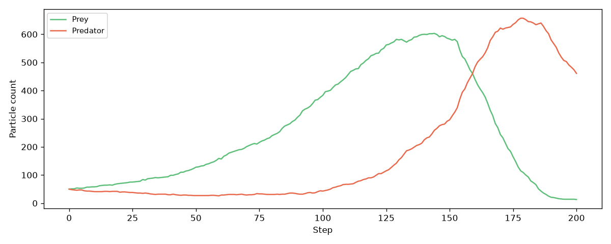
plot_species_counts() from plotting.py. Each frame on the x-axis is one batch of five steps.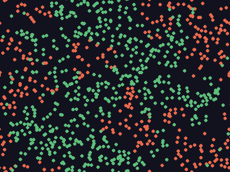
draw_frame() from drawing.py, just before the prey population collapses. The orange predators spread as fronts through the green prey.Notice also how long this tiny simulation took. When the populations boom to several hundred particles, apply_reactions() must consider every ordered pair of particles, and the number of pairs grows with the square of the number of particles. This is exactly the kind of computation that we would like to split across many processors.
Exercise: Modifyrun_serial.pyto load a different reaction file from thedatafolder, such asreactions_rps.csv(a rock-paper-scissors system with three species). Remember that the list of counts passed tomake_random_particles()needs one entry per species. Then useplot_species_counts()fromplotting.pyto save a chart of your run. How do the dynamics differ from predator and prey?
Looking ahead
This is the end of part one: we have a complete serial reaction-diffusion simulator that can handle any number of species, as long as each contact reaction involves two particles. Writing the parallel version might seem a little terrifying, since we know that it will be more complicated. Fortunately, we have done a lot of work that will help us, just as we did with our diffusion simulator. Functions like rand_step() and toroidal_distance() will come up again, and if we organize our parallel algorithm well, we can reuse much of what we have written. In the next code along, we will start building the parallel simulator by dividing the board into strips.