Code along video
Learning objectives
In this code along, we will plan our implementation of UPGMA from the top down. We will identify the data that we need to track, and then we will write the highest-level upgma() function, delegating every hard step to a subroutine that we will write in the next two code alongs.
Code along summary
Setup
To complete this code along, download the starter code as upgma-python.zip (found here), expand the folder, and move the resulting upgma directory into your python/src source code directory. The upgma directory has the following structure.
Data: a directory containing eight biological datasets, each in its own subfolder. Every subfolder includes a.mtxfile (the distance matrix that we will pass to UPGMA), anote.txtfile explaining where the data came from, and, where available, a.fastafile of the original sequences. We will explore these datasets once our implementation is finished.OutputandImages: initially empty directories where we will write our trees and pictures of them.datatypes.py: the data type declarations that we will use throughout this code along.functions.py: the file where we will implement UPGMA and all of its helper functions. Each function comes with a docstring and a body marked#TODO: Implementthat we will fill in.io_util.py: provided functions for reading a distance matrix from a.mtxfile and writing a tree to file.main.py: the file containingdef main(), which we will use for small experiments along the way and complete in a later code along.visualize_trees.R: an R script that we will use at the very end to draw our trees.
The data that UPGMA tracks
Let’s return to the example matrix on four species from the previous lesson, and think about which data our program will need to track as UPGMA runs.
First, we have the distance matrix, which shrinks by one row and column at each step. Second, we have the tree, which we represent as a list of nodes. If there are n species, then UPGMA takes n – 1 steps, adding one internal node at each step, so the tree will have n leaves and n – 1 internal nodes, or 2n – 1 nodes in total. Our plan is to create all 2n – 1 nodes at the start of the algorithm, with nodes 0 through n – 1 serving as the leaves. In our example, we will create seven nodes, numbered 0 through 6.
Third, we need a list that we will call clusters. At the start, row 0 of the matrix corresponds to node 0, row 1 corresponds to node 1, and so on. But as the algorithm runs, this correspondence breaks down; after the first step, row 2 of the matrix will correspond to the new internal node 4. The purpose of clusters is to tell us at any point in time which node of the tree each row of the matrix represents: row i of the matrix represents the cluster of leaves beneath the node clusters[i].
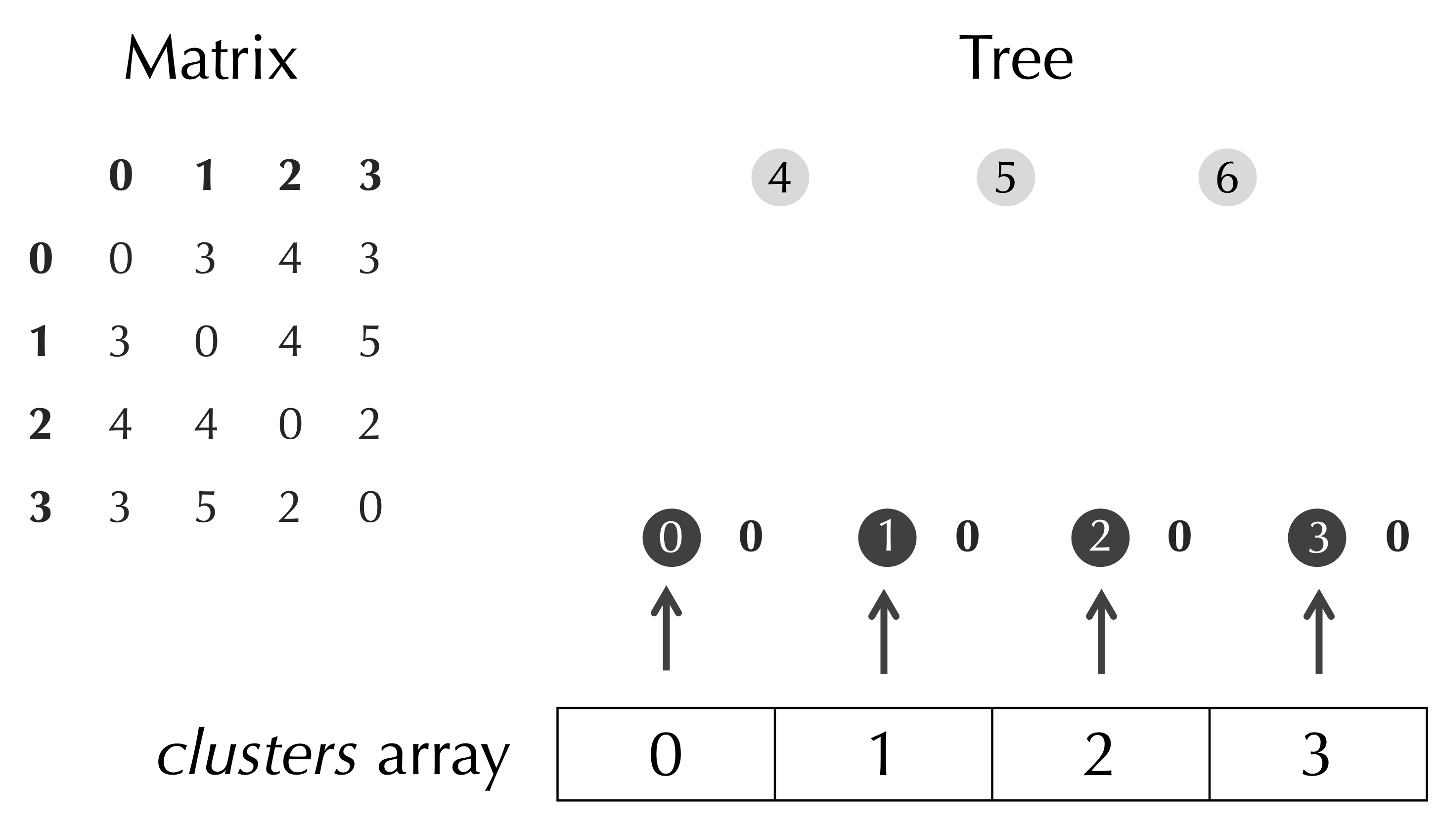
clusters refers to one of the leaves.Here is how these three data structures change at the first step of our example.
- The minimum element of the matrix is 2, at row 2 and column 3. We set the age of the current node, node 4, to 2/2 = 1, and we connect node 4 to its two children, which are
clusters[2]andclusters[3](nodes 2 and 3). - We add a new row and column to the matrix for the new cluster, whose values are the (weighted) averages of the values in rows 2 and 3. For example, the distance from row 0 to the new cluster is (4 + 3)/2 = 3.5.
- We delete the rows and columns at indices 2 and 3 of the matrix, which brings us down to a 3 × 3 matrix.
- We append node 4 to the end of
clusters, and then we delete the elements ofclustersat indices 2 and 3, the same indices that we deleted from the matrix. Nowclusterspoints at nodes 0, 1, and 4.
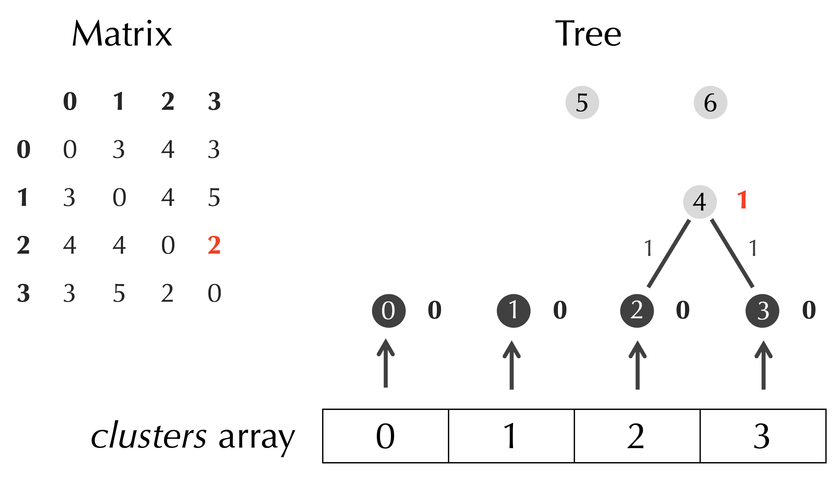
clusters[2] and clusters[3] and to give node 4 an age of 1.At the next step, the minimum element is 3, at row 0 and column 1, which means that we join clusters[0] and clusters[1] (here, nodes 0 and 1) under node 5. Then, at the final step, the minimum element is 4 at row 0 and column 1, and we join clusters[0] and clusters[1], which are now nodes 4 and 5, under node 6. At the end, the matrix has a single element, and clusters contains only the root.
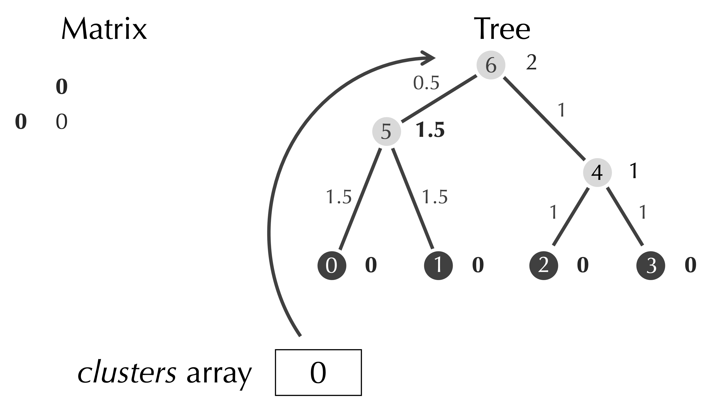
clusters contains a single element, which refers to the root, node 6.Note: The key pattern is that whenever the minimum element of the matrix is at rowrowand columncol, the children of the new node areclusters[row]andclusters[col]. The first time Phillip implemented UPGMA, he wrote out all of these steps by hand to make sure that he understood how the matrix, the tree, and the clusters connect. We recommend that you do the same.
Data types
Open datatypes.py. Our Node dataclass is the one that we designed in a previous code along, with an age attribute added. Each node has a label, an age, and references to its two children, which default to None. We will write its methods in a later code along.
@dataclass
class Node:
    label: str = "Unlabeled"
    age: float = 0.0
    child1: 'Node | None' = None
    child2: 'Node | None' = None
Previously, we declared Tree as a class whose only attribute was a list of nodes. When an object has only one attribute, though, we do not need a class at all. Instead, we will think of a tree as being defined by its list of nodes, using a type alias, just as we once declared a GameBoard to be a two-dimensional list when we worked with cellular automata. We will also declare a DistanceMatrix alias for a two-dimensional list of floats.
DistanceMatrix = list[list[float]]

Tree = list[Node]
UPGMA in pseudocode
The pseudocode for UPGMA fits on a single slide, with each subroutine that it calls written in bold below. This algorithm takes the idea of modularity to the extreme.
UPGMA(D, speciesNames)
    numLeaves ← CountRows(D)
    t ← InitializeTree(speciesNames)
    clusters ← InitializeClusters(t)
    for every integer p from numLeaves to 2*numLeaves-2
        row, col, val ← FindMinElt(D)
        t.nodes[p].age ← val/2
        t.nodes[p].child1 ← clusters[row]
        t.nodes[p].child2 ← clusters[col]
        clusterSize1 ← CountLeaves(t.nodes[p].child1)
        clusterSize2 ← CountLeaves(t.nodes[p].child2)
        D ← AddRowCol(D, clusterSize1, clusterSize2, row, col)
        D ← DelRowCol(D, row, col)
        clusters ← append(clusters, t.nodes[p])
        clusters ← DelClusters(clusters, row, col)
    return t
Writing upgma()
Open functions.py. The upgma() function takes a distance matrix and a list of species names, which we will use to label the leaves of the tree, and it returns a tree. (In our SARS-CoV-2 dataset, the species names will be sample dates, and in our bears dataset, they will be the names of bears.)
The first thing that we should do is make sure that our data are OK, since we will be reading matrices from many different files. There are many checks that we could perform, but two come to mind. First, a distance matrix with n rows should be a square n × n matrix. Second, the number of rows in the matrix should equal the number of species names. We will call a subroutine for each check.
def upgma(mtx: DistanceMatrix, species_names: list[str]) -> Tree:
    """
    Build a phylogenetic tree using the UPGMA algorithm.

    Given a distance matrix and species names, iteratively merges the closest
    clusters and updates the matrix using cluster-size-weighted averages.
    The resulting tree has `n` leaves (the species) and `n-1` internal nodes.

    Args:
        mtx (DistanceMatrix): Square symmetric matrix of pairwise distances.
        species_names (list[str]): Names of the species, in the same order as `mtx`.

    Returns:
        Tree: A list of `Node` objects representing the full UPGMA tree.
              Conventionally, the last node (index -1) is the root.
    """
    assert_square_matrix(mtx)
    assert_same_number_species(mtx, species_names)

    # we now know that the matrix is square, and that the number of rows is equal to the number of species
    num_leaves = len(mtx)
Once we have performed these checks, we know that the number of leaves is equal to both the number of rows in the matrix and the number of species names, so it does not matter which one we use for num_leaves.
Next, we make the tree, which will contain 2n – 1 nodes, with the leaves labeled by the species names. We will delegate this work to an initialize_tree() subroutine. Then we set clusters to refer to the first num_leaves nodes of the tree, which we can do with a slice, since a tree is just a list of nodes.
# make a tree containing 2n-1 total nodes, where the leaves are going to get labeled with species names
t = initialize_tree(species_names)

# clusters refer to the first num_leaves nodes in tree
clusters = t[:num_leaves]
STOP: This assignment toclusterslooks innocent. Can you think of anything that might cause it to produce a problem? We will answer this question in the next code along.
Next comes the engine of UPGMA, which runs for n – 1 steps, one for each internal node. The internal nodes have indices num_leaves up to (but not including) 2*num_leaves-1, so at each step, the current node is simply t[p]. Before writing any code inside the loop, we write a comment for each thing that needs to happen. And at the very end, we return the tree.
# perform the engine of UPGMA with n-1 total steps
# range over all the internal nodes and perform 1 step
for p in range(num_leaves, 2*num_leaves-1):
    # find minimum element of matrix

    # set the age of current node (t[p])

    # connect current node into its children

    # add a row and column to the matrix

    # delete the old rows/columns that are no longer needed

    # create a new cluster referring to the new node

    # delete the two clusters that we joined together

# return the tree
return t
Now we fill in each step, calling for help wherever we can.
- A
find_min_element()subroutine will return three things: the row index, the column index, and the value of the minimum element of the matrix. - The age of the current node is half of this minimum value.
- The hardest part of the algorithm is setting the children of
t[p]. As we saw in our example, they areclusters[row]andclusters[col]. Remember thatclustersis a list of nodes, so each of these is aNode. - When we add a row and column to the matrix, we need to compute a weighted average, and so we need to know the size of each cluster that we are joining. The size of a cluster is the number of leaves beneath its node in the tree. We will compute it with a
Nodemethod calledcount_leaves(), which we will write in a later code along. - Deleting rows and columns from the matrix is delegated to
delete_row_col(). - Creating a new cluster is just a matter of appending
t[p]toclusters. - Finally,
delete_clusters()will remove the two clusters at indicesrowandcol.
Here is our complete upgma() function.
def upgma(mtx: DistanceMatrix, species_names: list[str]) -> Tree:
    """
    Build a phylogenetic tree using the UPGMA algorithm.

    Given a distance matrix and species names, iteratively merges the closest
    clusters and updates the matrix using cluster-size-weighted averages.
    The resulting tree has `n` leaves (the species) and `n-1` internal nodes.

    Args:
        mtx (DistanceMatrix): Square symmetric matrix of pairwise distances.
        species_names (list[str]): Names of the species, in the same order as `mtx`.

    Returns:
        Tree: A list of `Node` objects representing the full UPGMA tree.
              Conventionally, the last node (index -1) is the root.
    """
    assert_square_matrix(mtx)
    assert_same_number_species(mtx, species_names)

    # we now know that the matrix is square, and that the number of rows is equal to the number of species
    num_leaves = len(mtx)

    # make a tree containing 2n-1 total nodes, where the leaves are going to get labeled with species names
    t = initialize_tree(species_names)

    # clusters refer to the first num_leaves nodes in tree
    clusters = t[:num_leaves]

    # perform the engine of UPGMA with n-1 total steps
    # range over all the internal nodes and perform 1 step
    for p in range(num_leaves, 2*num_leaves-1):
        # find minimum element of matrix
        row, col, min_val = find_min_element(mtx)

        # set the age of current node (t[p])
        t[p].age = min_val/2.0

        # connect current node into its children
        t[p].child1 = clusters[row]  # this is a Node!
        t[p].child2 = clusters[col]

        # add a row and column to the matrix

        cluster_size_1 = t[p].child1.count_leaves()
        cluster_size_2 = t[p].child2.count_leaves()

        mtx = add_row_col(row, col, cluster_size_1, cluster_size_2, mtx)

        # delete the old rows/columns that are no longer needed

        mtx = delete_row_col(mtx, row, col)

        # create a new cluster referring to the new node
        clusters.append(t[p])

        # delete the two clusters that we joined together
        clusters = delete_clusters(clusters, row, col)

    # return the tree
    return t
Note: In the video, the call toadd_row_col()is typed withmtxas its first argument. The code above passes the arguments in the order given by theadd_row_col()signature in the starter code,(row, col, cluster_size1, cluster_size2, mtx), which is also the order used in the video when the code is run in a later code along.
Our function is short, but it calls eight subroutines, and it does so in a coordinated way because we understood the algorithm before we wrote any code. What is left is to write these subroutines.
Looking ahead
In the next code along, we will write our functions that validate the input and initialize the tree. We will also answer our question about whether clusters = t[:num_leaves] causes a problem, which will require us to understand exactly what a slice copies.