Learning objectives
In this code along, we will build a physics engine to simulate the force of gravity and how it affects the motions of a collection of heavenly bodies, solving the problem below whose solution we discussed in a language-neutral fashion in the core text. We will then run this simulation on the moons of Jupiter as well as a collection of three-body simulations that exhibit beautiful patterns.
Gravity Simulator Problem
Input: A Universe object initialUniverse, an integer numGens, and a floating-point number time.
Output: An array timePoints of numGens + 1 Universe objects, where timePoints[0] is initialUniverse, and timePoints[i] is obtained from timePoints[i-1] by approximating the results of the force of gravity over a time interval equal to time (in seconds).
Setup
To complete this code along, we will need starter code that handles file I/O, drawing, and animation — allowing us to focus on the physics engine itself.
We provide this starter code as a single download gravity.zip. Download this code here, and then expand the folder. Move the resulting gravity directory into your python/src source code directory.
The gravity directory has the following structure:
data: a directory containing.txtfiles that represent different initial systems that we will simulate.output: an initially empty directory that will contain images and .mp4 videos that we draw.datatypes.py: a file where we will define our dataclass declarations.gravity.py: a file where we will implement our physics engine. This is the main focus of this code along.custom_io.py: a provided file that contains code for reading in a system of heavenly bodies from file.drawing.py: a provided file that contains code for drawing a system to an image and creating animations over multiple time steps.animate.py: a provided file that converts a list ofpygame.Surfaceobjects into an MP4 video.main.py: a file that will containdef main(), where we will call functions to read in systems, run our gravity simulation, and draw the results.
Here is what our main() contains at the start of this code along.
def main():
    print("Building a gravity simulator.")

if __name__ == "__main__":
    main()
Code along summary
Organizing data
We begin with datatypes.py, which will store all our class declarations. As we saw in the core text, in the same way that we design functions top-down, we can design objects top-down as well. We recall the language-neutral type declarations for our gravity simulator below, starting with a Universe object, which contains an array of Body objects as one of its fields.
type Universe
    bodies []Body
    width float
    gravitationalConstant float
In turn, we define a Body object, which includes multiple fields involving OrderedPair objects, as shown below.
type Body
    name string
    mass float
    radius float
    position OrderedPair
    velocity OrderedPair
    acceleration OrderedPair
    red int
    green int
    blue int

type OrderedPair
    x float
    y float
To implement these ideas, we will apply what we learned in the previous code along about dataclasses. We start with the OrderedPair dataclass, which we already defined previously.
from dataclasses import dataclass, field

@dataclass
class OrderedPair:
    x: float = 0.0
    y: float = 0.0
Next, we define our Body dataclass, where the position, velocity, and acceleration attributes are each represented by an OrderedPair object. Recall that we use field(default_factory=OrderedPair) for mutable defaults so that each Body gets its own independent objects. We also add red, green, and blue fields for the body’s color.
@dataclass
class Body:
    name: str = ""
    mass: float = 0.0
    position: OrderedPair = field(default_factory=OrderedPair)
    velocity: OrderedPair = field(default_factory=OrderedPair)
    acceleration: OrderedPair = field(default_factory=OrderedPair)
    radius: float = 0.0
    red: int = 0
    green: int = 0
    blue: int = 0
Finally, we define our Universe dataclass, which contains a list of Body objects, a width (in meters) for establishing the boundaries of a square region that we will render, and a gravitational constant. Note that bodies uses field(default_factory=list) rather than a plain = [] because lists are mutable, and without this specification, every instance of a Universe object would share the same list.
@dataclass
class Universe:
    bodies: list[Body] = field(default_factory=list)
    width: float = 1000.0
    gravitational_constant: float = 6.674e-11
Reading a universe from file
The data directory contains a collection of plain text files, one for each universe that we will model. For example, the figures below show butterfly.txt on the left (which represents a three-body system) and the first 20 lines of jupiter_moons.txt on the right (which represents Jupiter and four moons).
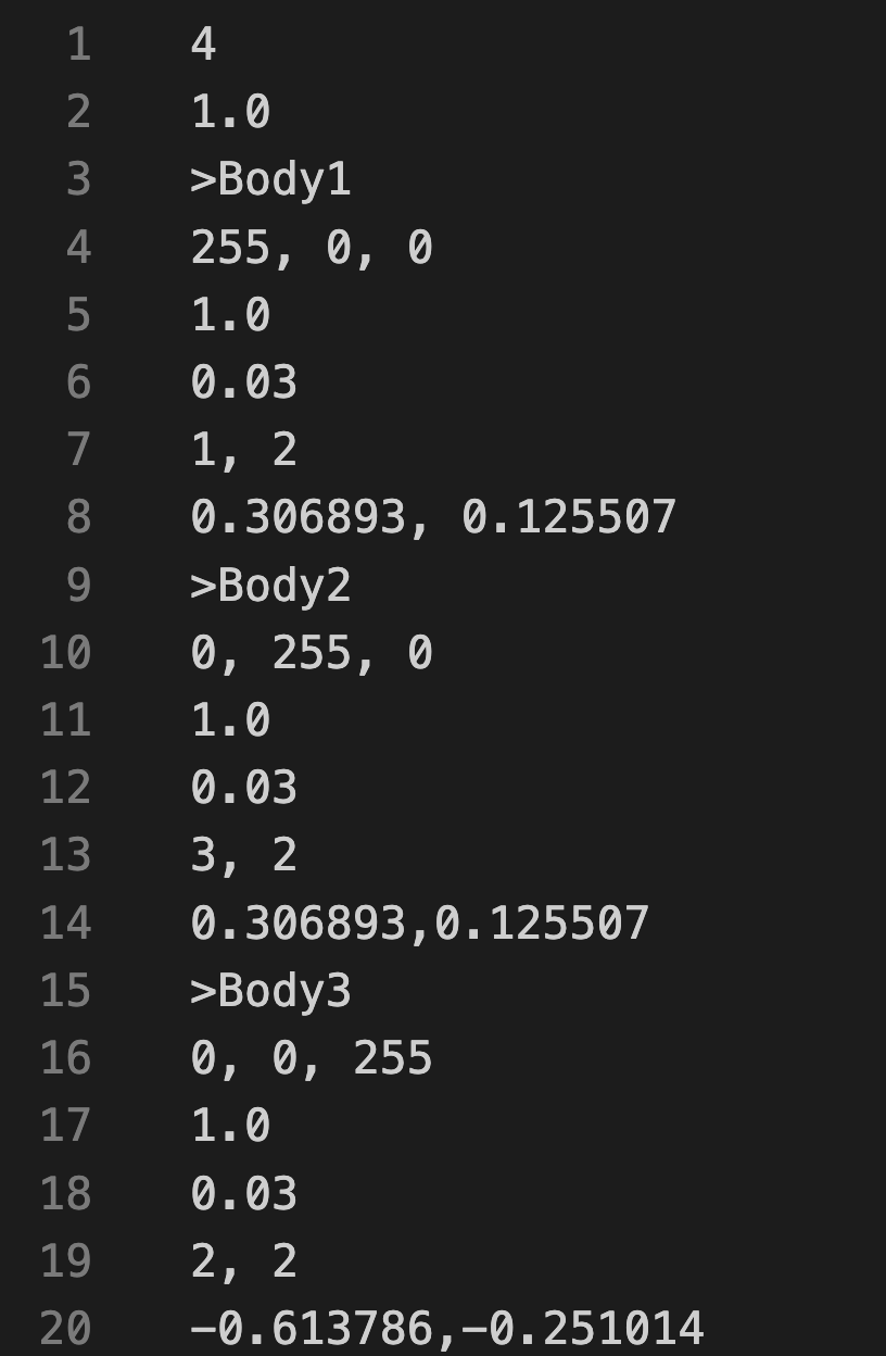
a universe width of 4 meters. Each body block specifies a name (prefixed by >), an RGB color, a mass
(kg), a radius (m), an initial position (m), and an initial velocity (m/s).
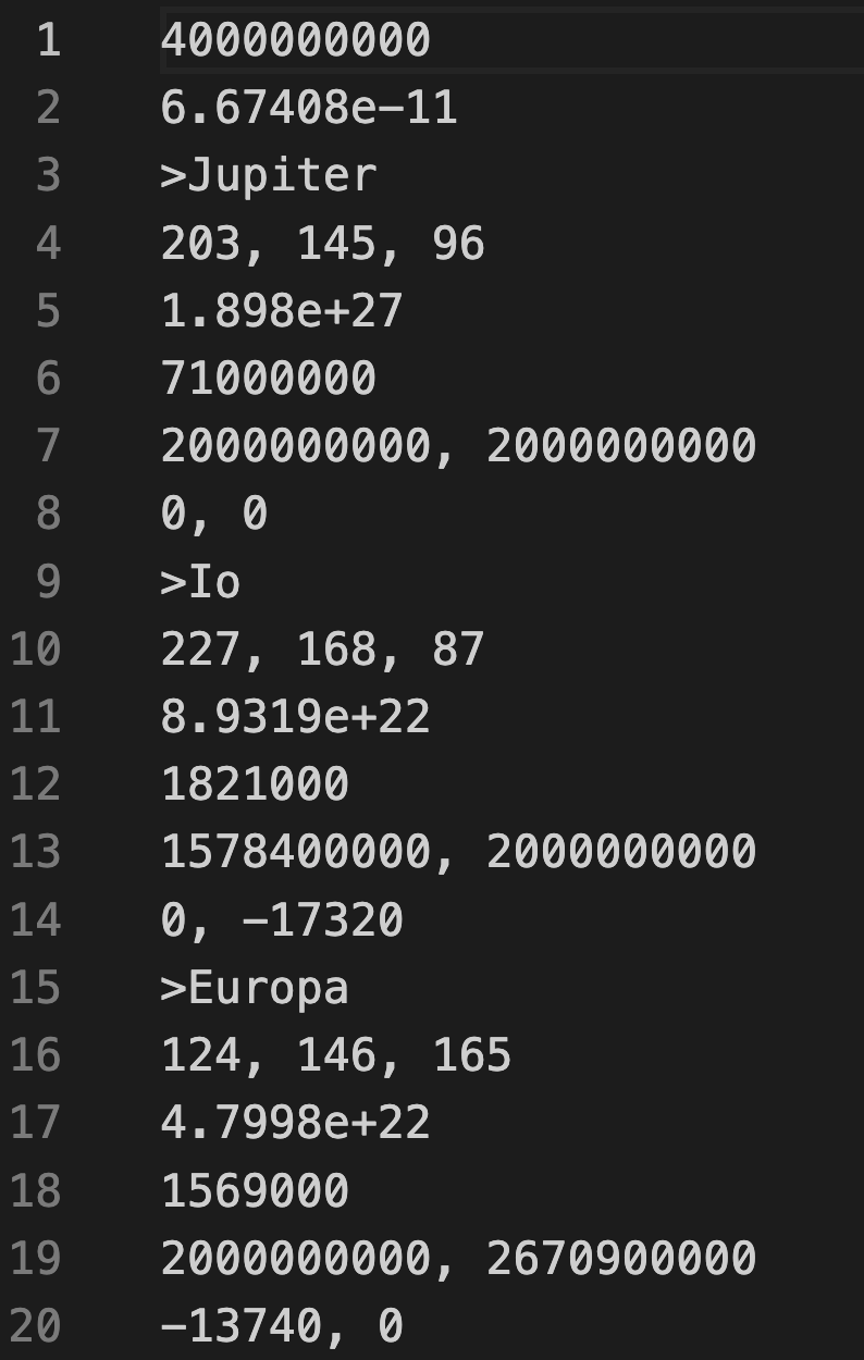
physical values. The universe width is 4 billion meters and the gravitational constant is the standard
SI value. Positions and velocities are drawn from orbital data.
The first line of each universe data file specifies the width of the universe, and the second line stores the gravitational constant. The bodies of the universe are then given in subsequent blocks, where each block consists of six lines:
- Name of the body
- RGB color (three integers in the range 0–255)
- Mass (in kg)
- Radius (in m)
- Initial position components (x, y)
- Initial velocity components (vx, vy)
Note that the gravitational constant for butterfly.txt (and in fact all the three-body systems in our example) is standardized to 1 to allow the simulation values to be somewhat small; they could be scaled up to have the same gravitational constant as is observed in our universe.
Our primary function in custom_io.py is read_universe(), which takes as input a string filename. This function parses the file contained at the location given by filename into a Universe object that it returns. This function, along with two subroutines that it calls, is provided in the starter code.
Starting our highest level function
Now we turn to gravity.py, where we will implement our physics engine. First, we will implement our highest level function, which will solve the Gravity Simulator Problem; its pseudocode representation from the core text is shown below.
SimulateGravity(initialUniverse, numGens, time)
    timePoints ← array of numGens+1 Universe objects
    timePoints[0] ← initialUniverse
    for every integer i between 1 and numGens
        timePoints[i] ← UpdateUniverse(timePoints[i-1], time)
    return timePoints
This function is an easy one to write, since we are being lazy as always and passing the work to an update_universe() subroutine. We add a few parameter checks at the top to validate our inputs before entering the simulation loop.
def simulate_gravity(initial_universe: Universe, num_gens: int, time: float) -> list[Universe]:
    """
    Simulate an N-body system for a fixed number of generations.

    Args:
        initial_universe: The starting state of the universe.
        num_gens: Number of simulation steps to advance (>= 0).
        time: Time step (Δt) between generations (> 0).

    Returns:
        A list of Universe snapshots of length num_gens + 1.
    """
    if not isinstance(initial_universe, Universe):
        raise TypeError("initial_universe must be a Universe")
    if not isinstance(num_gens, int) or num_gens < 0:
        raise ValueError("num_gens must be a non-negative integer")
    if not isinstance(time, (int, float)) or time <= 0:
        raise ValueError("time must be a positive number")

    time_points: list[Universe] = [initial_universe]

    for i in range(1, num_gens + 1):
        next_universe = update_universe(time_points[i - 1], time)
        time_points.append(next_universe)

    return time_points
Updating a universe
Our update_universe() function advances the state of every Body in the universe by one time step. It creates a deep copy of the current universe (we will explain why in a moment), and then updates each body’s acceleration, velocity, and position in that copy, delegating each computation to a subroutine.
def update_universe(current_universe: Universe, time: float) -> Universe:
    """
    Advance the universe by a single time step.
    Computes new accelerations from the current state, then advances velocity and position accordingly.

    Args:
        current_universe: Universe state at the current time.
        time: Time step (Δt) to advance.

    Returns:
        A new Universe instance representing the next state.
    """
    new_universe = copy_universe(current_universe)

    # Update every body in the cloned universe based on forces from current_universe
    for b in new_universe.bodies:
        old_acc, old_vel = b.acceleration, b.velocity
        b.acceleration = update_acceleration(current_universe, b)
        b.velocity = update_velocity(b, old_acc, time)
        b.position = update_position(b, old_acc, old_vel, time)

    return new_universe
Copying a universe
You might wonder why we cannot simply write new_universe = current_universe to obtain a copy of the existing Universe object. The answer is that Python objects are passed by reference: that assignment does not create a new Universe; rather, it creates a second name that points to the same object in memory. Any change we make to a Body inside new_universe would silently modify current_universe as well. To avoid this, we need a deep copy: a completely independent Universe object whose Body objects and OrderedPair objects are all freshly allocated. (We will say more about deep copies in the next chapter.)
We now write copy_universe() and its helper copy_body(). Note how copy_universe() delegates each body’s copy to copy_body().
Note: In future code alongs, we will show how to perform a deep copy without having to write our own functions.
def copy_universe(current_universe: Universe) -> Universe:
    """
    Deep-copy a Universe, including all of its bodies.

    Args:
        current_universe: The universe to copy.

    Returns:
        A new Universe with deep-copied bodies and the
        same width and gravitational constant as the original.
    """
    new_bodies: list[Body] = []

    for b in current_universe.bodies:
        new_bodies.append(copy_body(b))

    return Universe(
        new_bodies,
        current_universe.width,
        current_universe.gravitational_constant,
    )

def copy_body(b: Body) -> Body:
    """
    Deep-copy a Body, including its position, velocity, and acceleration.

    Args:
        b: The body to copy.

    Returns:
        A new Body with identical attributes and
        deep-copied OrderedPair objects.
    """
    return Body(
        name=b.name,
        mass=b.mass,
        position=OrderedPair(b.position.x, b.position.y),
        velocity=OrderedPair(b.velocity.x, b.velocity.y),
        acceleration=OrderedPair(b.acceleration.x, b.acceleration.y),
        radius=b.radius,
        red=b.red,
        green=b.green,
        blue=b.blue,
    )
Using Newton’s laws to compute the net force (acceleration) on a body
update_acceleration() computes the new acceleration of a body by first finding the net gravitational force acting on it, then applying Newton’s second law: a = F / m. It delegates the force calculation to compute_net_force(), which we will write next.
def update_acceleration(current_universe: Universe, b: Body) -> OrderedPair:
    """
    Compute a body's acceleration from the net gravitational force.

    Args:
        current_universe: The universe containing all bodies.
        b: The body whose acceleration is being computed.

    Returns:
        An OrderedPair (ax, ay) representing the updated acceleration.
    """
    net_force = compute_net_force(current_universe, b)

    # apply Newton's second law over components
    ax = net_force.x / b.mass
    ay = net_force.y / b.mass

    return OrderedPair(ax, ay)
The net gravitational force on a body is the vector sum of the individual forces exerted on it by every other body in the universe. compute_net_force() loops over all bodies in the universe, skips the body itself (a body does not exert a gravitational force on itself), and accumulates the x- and y-components of each pairwise force, delegating each pairwise calculation to compute_force().
def compute_net_force(current_universe: Universe, b: Body) -> OrderedPair:
    """
    Compute the net gravitational force on a body from all other bodies.

    Args:
        current_universe: The universe containing all bodies.
        b: The body on which the net force is computed.

    Returns:
        An OrderedPair (Fx, Fy) representing the net gravitational force.
    """
    net_force = OrderedPair(0.0, 0.0)

    G = current_universe.gravitational_constant

    # range over bodies and determine force acting on b
    for cur_body in current_universe.bodies:
        if cur_body is not b:
            current_force = compute_force(b, cur_body, G)
            net_force.x += current_force.x
            net_force.y += current_force.y

    return net_force
The pairwise gravitational force between two bodies is given by Newton’s law of universal gravitation: F = G · m1 · m2 / d2, directed from b1 toward b2. compute_force() computes this magnitude and then decomposes it into x and y components by multiplying by the unit vector pointing from b1 to b2. Note that we handle the edge case of two bodies occupying exactly the same position by returning a zero force, which avoids a division-by-zero error.
def compute_force(b1: Body, b2: Body, G: float) -> OrderedPair:
    """
    Compute the gravitational force exerted on b1 by b2.

    Args:
        b1: The body on which the force is acting.
        b2: The body exerting the gravitational force.
        G: Gravitational constant.

    Returns:
        An OrderedPair (Fx, Fy) representing the force on b1.
    """
    d = distance(b1.position, b2.position)

    if d == 0.0:
        return OrderedPair(0.0, 0.0)  # treat as no force

    F_magnitude = G * b1.mass * b2.mass / (d * d)

    # break F into components
    dx = b2.position.x - b1.position.x
    dy = b2.position.y - b1.position.y
    Fx = F_magnitude * dx / d
    Fy = F_magnitude * dy / d

    return OrderedPair(Fx, Fy)
The computation of force requires knowing the distance between two bodies. We compute this using the standard Euclidean distance formula, which is its own small but reusable subroutine.
def distance(p1: OrderedPair, p2: OrderedPair) -> float:
    """
    Compute the Euclidean distance between two position vectors.

    Args:
        p1: The first position vector.
        p2: The second position vector.

    Returns:
        The distance between p1 and p2.
    """
    dx = p2.x - p1.x
    dy = p2.y - p1.y

    return math.sqrt(dx * dx + dy * dy)
Updating the velocity and position of a body
We update the velocity of a body using the velocity-Verlet method, which averages the old and new accelerations over the time step. This gives a more accurate result than simply using either the old or the new acceleration alone, and is a standard technique in physics simulations. Note that by the time update_velocity() is called from update_universe(), b.acceleration has already been updated to the new value, which is why we also pass the old acceleration as a separate argument.
def update_velocity(b: Body, old_acceleration: OrderedPair, time: float) -> OrderedPair:
    """
    Update velocity using average acceleration over the step.

    Formula:
        v_{t+Δt} = v_t + 0.5 * (a_t + a_{t+Δt}) * Δt

    Args:
        b: The body whose velocity is being updated.
        old_acceleration: The acceleration at the previous time step.
        time: The time step Δt.

    Returns:
        An OrderedPair containing the updated velocity (vx, vy).
    """
    vx = b.velocity.x + 0.5 * (b.acceleration.x + old_acceleration.x) * time
    vy = b.velocity.y + 0.5 * (b.acceleration.y + old_acceleration.y) * time

    return OrderedPair(vx, vy)
We update position using the standard kinematic formula, which accounts for both the initial velocity and the acceleration over the time interval. We use the old velocity and old acceleration here, which is why update_universe() saves them explicitly before calling update_acceleration().
def update_position(b: Body, old_acc: OrderedPair, old_vel: OrderedPair, time: float) -> OrderedPair:
    """
    Update position using constant-acceleration kinematics.

    Formula:
        p_{t+Δt} = p_t + v_t * Δt + 0.5 * a_t * Δt²

    Args:
        b: The body whose position is being updated.
        old_acc: The acceleration at the previous time step.
        old_vel: The velocity at the previous time step.
        time: The time step Δt.

    Returns:
        An OrderedPair containing the updated position (px, py).

    """
    px = b.position.x + old_vel.x * time + 0.5 * old_acc.x * time * time
    py = b.position.y + old_vel.y * time + 0.5 * old_acc.y * time * time

    return OrderedPair(px, py)
Running the simulation
Now that we have implemented our physics engine, we can write main() to tie everything together. Our program will read five command-line arguments: the scenario name (matching a .txt file in the data/ directory), the number of simulation generations, the time step in seconds, the canvas width in pixels, and a drawing frequency that controls how often we render a frame (we only produce a surface for every drawing_frequency-th time step, which allows us to run many more total generations while keeping the output video a manageable length). Here is the complete main().
def main():
    print("Let's simulate gravity!")

    # Expect 5 user arguments (plus program name)
    if len(sys.argv) != 6:
        raise ValueError(
            "Error: incorrect number of command line arguments. Six desired."
        )

    scenario = sys.argv[1]

    # establish input file and output prefix
    input_file = f"data/{scenario}.txt"
    video_path = f"output/{scenario}.mp4"

    # Parse CLI arguments
    num_gens = int(sys.argv[2])
    time_step = float(sys.argv[3])
    canvas_width = int(sys.argv[4])
    drawing_frequency = int(sys.argv[5])
    print("Command line arguments read!")

    # Read initial universe
    initial_universe = read_universe(input_file)

    print("Simulating gravity now.")
    time_points = simulate_gravity(initial_universe, num_gens, time_step)
    print("Gravity simulation complete.")

    print("Rendering frames.")
    surfaces = animate_system(time_points, canvas_width, drawing_frequency)
    print("Frames drawn.")

    print("Encoding MP4 video.")
    animate_surfaces(surfaces, path)
    print("Success! MP4 video produced.")
    print("Animation finished! Exiting normally.")
Let’s start by running the simulation on the Jupiter moons system. The command below simulates 1,000 generations with a time step of 60 seconds (one minute per step), a canvas 1,500 pixels wide, and a drawing frequency of 10 (so that we capture one frame for every 10 simulation steps).
STOP: In a new terminal window, navigate into our directory usingcd python/src/gravity. Then run the command below.
python3 main.py jupiter_moons 1000 60 1500 10
Once you have verified that your code is working, try changing the gravitational constant in jupiter_moons.txt — double it, halve it, or experiment with other values. Notice how the orbital periods and trajectories change: a stronger gravitational constant pulls the moons into tighter, faster orbits, while a weaker one causes them to drift more slowly.
Three-body simulations
Now for the main event. Our data/ directory includes several classic three-body initial conditions. Unlike the Jupiter system, these simulations use a gravitational constant of 1 and much smaller time steps, since the bodies are much lighter and closer together relative to their masses. Three-body orbits are also famously unstable: small numerical errors accumulate over time and the bodies eventually diverge from their ideal trajectories, so we need many more generations at a finer time step to capture the full pattern before chaos sets in. The commands below each take about 30 seconds to run.
python3 main.py butterfly 100000 0.0001 1500 300
python3 main.py dragonfly 100000 0.0001 1500 300
python3 main.py figure_eight 100000 0.0001 1500 300
python3 main.py goggles 100000 0.0001 1500 300
python3 main.py moth 100000 0.0001 1500 300
python3 main.py yarn 100000 0.0001 1500 300
For even higher resolution and smoother trails, we can simulate ten times as many generations with a proportionally smaller time step. These runs will take longer but produce the most visually striking results.
python3 main.py butterfly 1000000 0.00001 1500 3000
python3 main.py dragonfly 1000000 0.00001 1500 3000
After running these simulations, you will find the following videos in your output/ directory. The provided drawing.py includes trail visualization, which traces the path each body has traveled through space and reveals the beautiful structure of these choreographed orbits.
The dragonfly three-body orbit:
The butterfly three-body orbit:
Time for practice!
After you have the chance to check your work below, you are ready to apply what you have learned to the chapter’s practice problems. Or, you can carry on to the next chapter, where we will learn about how to construct evolutionary trees from DNA data.