Chapter 4 Practice Exercises: Boids!

An introduction to the boids simulation

Birds are able to fly in a flock and change directions in response to their environment despite not having any central coordination or higher intelligence. Yet for many years, graphics designers struggled to build algorithms simulating birds’ collective movement.

In this assignment, you will build a landmark “artificial life” flocking algorithm called boids that was developed in 1986 by Craig Reynolds (citation: https://doi.org/10.1145/37401.37406). The first publicly available animation of this flock algorithm is shown below.

As you will see, the simulation produced by this algorithm is beautiful, and yet it can be summarized in three simple principles followed by every boid in the simulation.

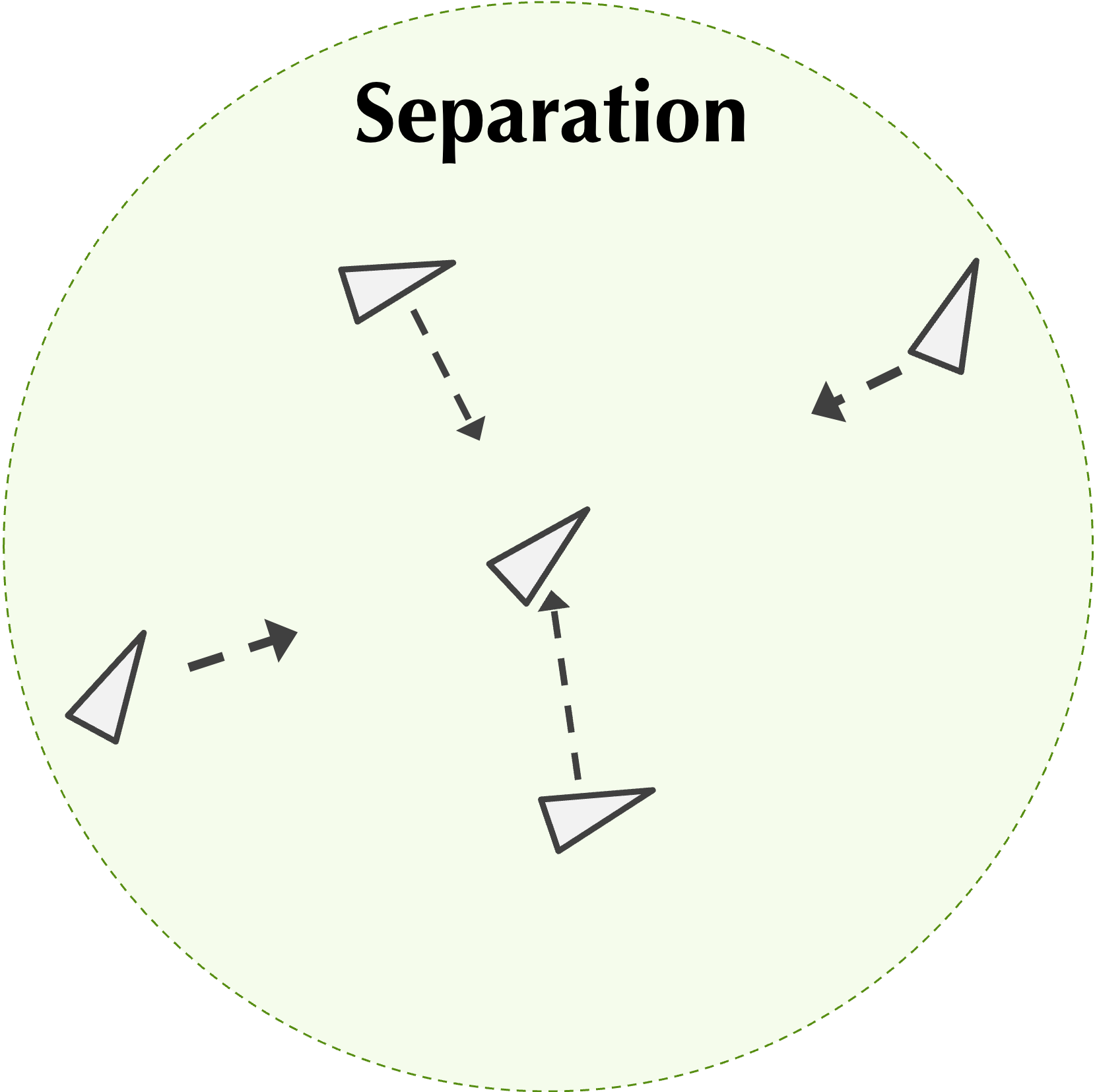
1. Separation: boids try to avoid collisions with other nearby boids.
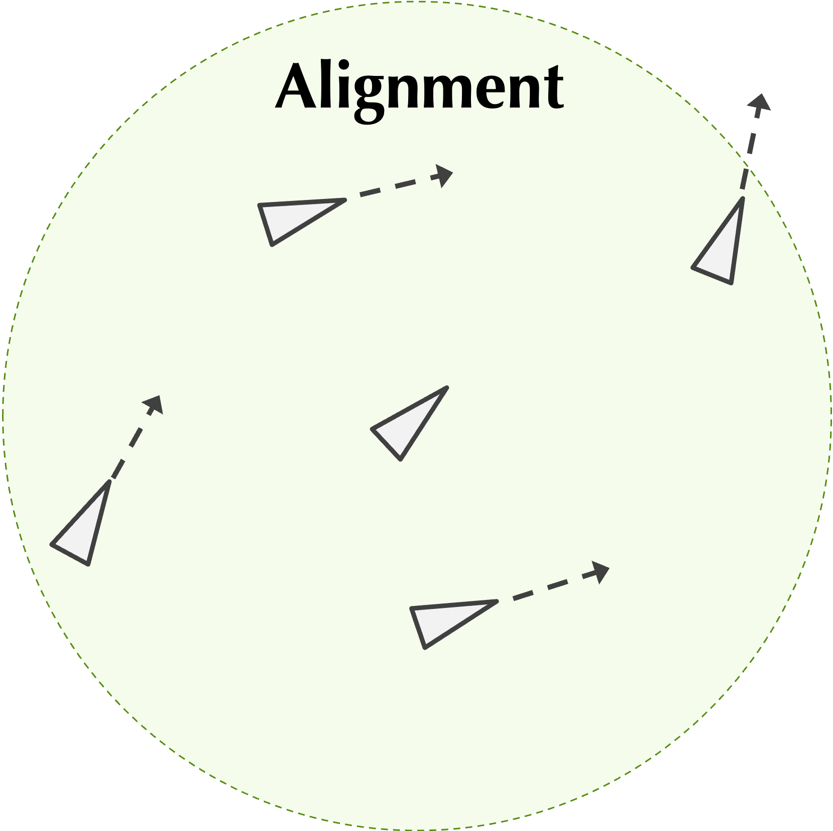
2. Alignment: boids try to match the velocities of nearby boids.
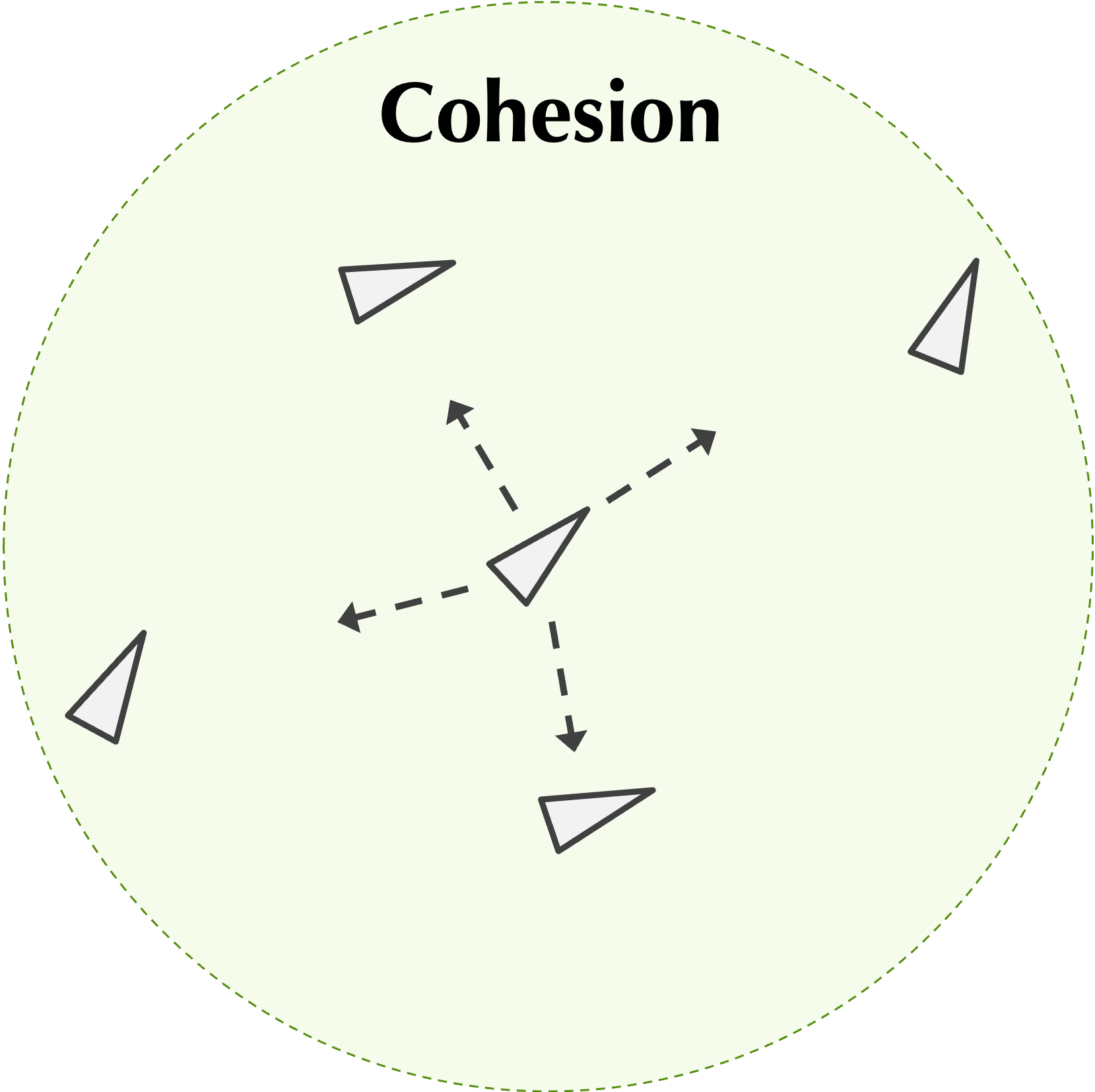
3. Cohesion: boids try to remain close to nearby boids, which keeps the flock together.

All three rules are distributed, meaning that each boid changes its behavior independently of other boids. Furthermore, none of these three rules requires any intelligence on behalf of the boids. We will illustrate these three rules on the following steps.

Learning objectives

By completing this assignment, you will be able to:

• Adapt a given physics simulation (gravity) into a new context (flocking).
• Apply object-oriented programming to represent agents and their environment.
• Appreciate how complex behavior can emerge from simple rules.
• Recognize that many natural algorithms are distributed: each agent has limited information, yet global patterns arise.

Computations of the three boid forces

We previously built a gravity simulation over a collection of small discrete time step snapshots. We will apply this same model to simulating a system of boids, which is more similar to a gravitational simulation than you might at first think because each of the three rules can be represented by “forces” driving the boids’ behavior.

Each of the three rules will only be applied if two boids are within a threshold distance. That is, for some global parameter of the system d_threshold, we will only apply the force if the distance d between two boids is strictly less than d_threshold. (We apply this for consistency and could change the specification to if d is less than or equal to d_threshold without much change in the resulting animations.)

We also should specify that if the distance between two boids d is precisely equal to zero, then we will not model a collision between the two boids. However, the forces below all involve a division by d, so to handle the case when the two boids occupy the same position, we will not compute a force between them.

Computing the force due to separation

We will examine how each of the three rules can be implemented, beginning with the “separation” rule, whose figure is reproduced below. When working with gravity, we assumed that objects are attracted to each other with a force that is inversely proportional to the square of the distance between them. As a result, the force of gravity dissipates quickly as two objects grow distant from each other.

In the boid simulation, we will assume that the separation force causes objects to be repelled by a force that is inversely proportional to the distance between them (and that the force is zero once the boids are outside a threshold distance).

In other words, if boids b1 and b2 are within a critical distance of each other and have positions (x₁, y₁) and (x₂, y₂), then the force acting on b1 due to the separation force with b2 has components given by

F_x = c_\text{separation} \cdot (x_1 - x_2)/d^2\\ F_y = c_\text{separation} \cdot (y_1 - y_2)/d^2

Here, c_separation is a constant called the separation factor that helps dictate the magnitude of the separation force.

For a given boid b, after determining the force due to separation exerted on b by each boid within a threshold distance of b, we take the average of all these forces to obtain a final force acting on b due to separation.

Computing the force due to alignment

Next, we will consider the “alignment” rule, which states that boids will match the velocities of nearby boids. To translate this rule into forces, we will convert each boid’s velocity as a force pulling other nearby boids in the direction of this velocity.

In one extreme case, two nearby boids are traveling in opposite directions, and so their velocity vectors will cancel. In another extreme case, every nearby boid is traveling in the same direction, and so these boids should pull along a given boid.

To determine the force due to alignment acting on boid b1 due to a nearby boid b2, say that the velocity of b2 is given by the vector (v_x, v_y). Then for some constant c_alignment called the alignment factor, the force acting on b1 due to b2 as a result of alignment has the following components:

F_x = c_\text{alignment} \cdot v_x / d\\ F_y = c_\text{alignment} \cdot v_y / d

As with the separation force, for a given boid b, after determining the alignment force exerted on b by each boid within a threshold distance of b, we take the average of all these forces to obtain a final force acting on b due to alignment.

Computing the force due to cohesion

Finally, we consider the “cohesion” principle, which states that nearby boids tend to stick together. At first glance, this rule may seem at odds with the “separation” rule. However, the repellent force due to separation increases as two boids get closer; in contrast, the attractive force due to cohesion will be constant for all boids that are within the threshold distance. The combination of the cohesion and separation forces will therefore cause a rubber band effect, in which two boids will be attracted to each other by the cohesion force but will then be repelled by the increasing separation force.

If boids b1 and b2 are within the threshold distance of each other and have positions (x₁, y₁) and (x₂, y₂), then for some constant c_cohesion called the cohesion factor, the force acting on b1 due to cohesion with b2 has components given by

F_x = c_\text{cohesion} \cdot (x_2 - x_1)/d\\ F_y = c_\text{cohesion} \cdot (y_2 - y_1)/d

Once again, for a given boid b, after determining the cohesion force acting on b by every other boid within a threshold distance, we take the average of all these forces to obtain a final force acting on b due to cohesion.

Updating a boid’s acceleration

Once we have determined the force acting on a boid as the result of separation, alignment, and cohesion, we can sum these forces (componentwise) to obtain the net force acting on the boid.

We would like to convert this net force into a net acceleration, and to simplify our computations, we will assume that boids have unit mass. Recall that by Newton’s second law, the force F acting on an object is subject to the equation F = m · a, where m is the mass of the object and a is its acceleration. As a result, if m is equal to 1, then F and a have the same values (although the units will be different).

In any of the boid simulation rules, if there are no boids within the given threshold distance of a boid, then the net force acting on that boid should be zero. Make sure to handle this case so that you don’t wind up dividing by zero!

Updating a boid’s velocity and position

When updating the velocity and position of a boid, we will use the same dynamics equations that we used in our gravity simulation, which are reproduced below.

In particular, let (p_x(n), p_y(n)), (v_x(n), v_y(n)), and (a_x(n), a_y(n)) denote the position, velocity, and acceleration in generation n, respectively, and let t denote the time interval between generations. The velocity vector (v_x(n+1), v_y(n+1)) in generation n+1 is given by the following:

v_x(n+1) = \tfrac{1}{2} \cdot \left(a_x(n) + a_x(n+1)\right) \cdot t + v_x(n)\\ v_y(n+1) = \tfrac{1}{2} \cdot \left(a_y(n) + a_y(n+1)\right) \cdot t + v_y(n)\\[1em] p_x(n+1) = \tfrac{1}{2} \cdot a_x(n) \cdot t^2 + v_x(n) \cdot t + p_x(n)\\ p_y(n+1) = \tfrac{1}{2} \cdot a_y(n) \cdot t^2 + v_y(n) \cdot t + p_y(n)

In addition to applying the dynamics equations from the previous step, our boids simulation has two additional features.

Limiting boid speed

Because boids are intended to model birds, we will ensure that boids cannot fly too fast. To do so, we will have an additional parameter maxBoidSpeed representing the maximum speed of any boid.

The speed of a boid whose velocity components are given by (v_x(t), v_y(t)) is equal to

s = \sqrt{v_x(t)^2 + v_y(t)^2}

In each time step, if the speed s of a boid is greater than maxBoidSpeed, then we will lower the boid’s velocity by multiplying both v_x(t) and v_y(t) by maxBoidSpeed/s. (If s is smaller than maxBoidSpeed, then we do not adjust the boid’s velocity.)

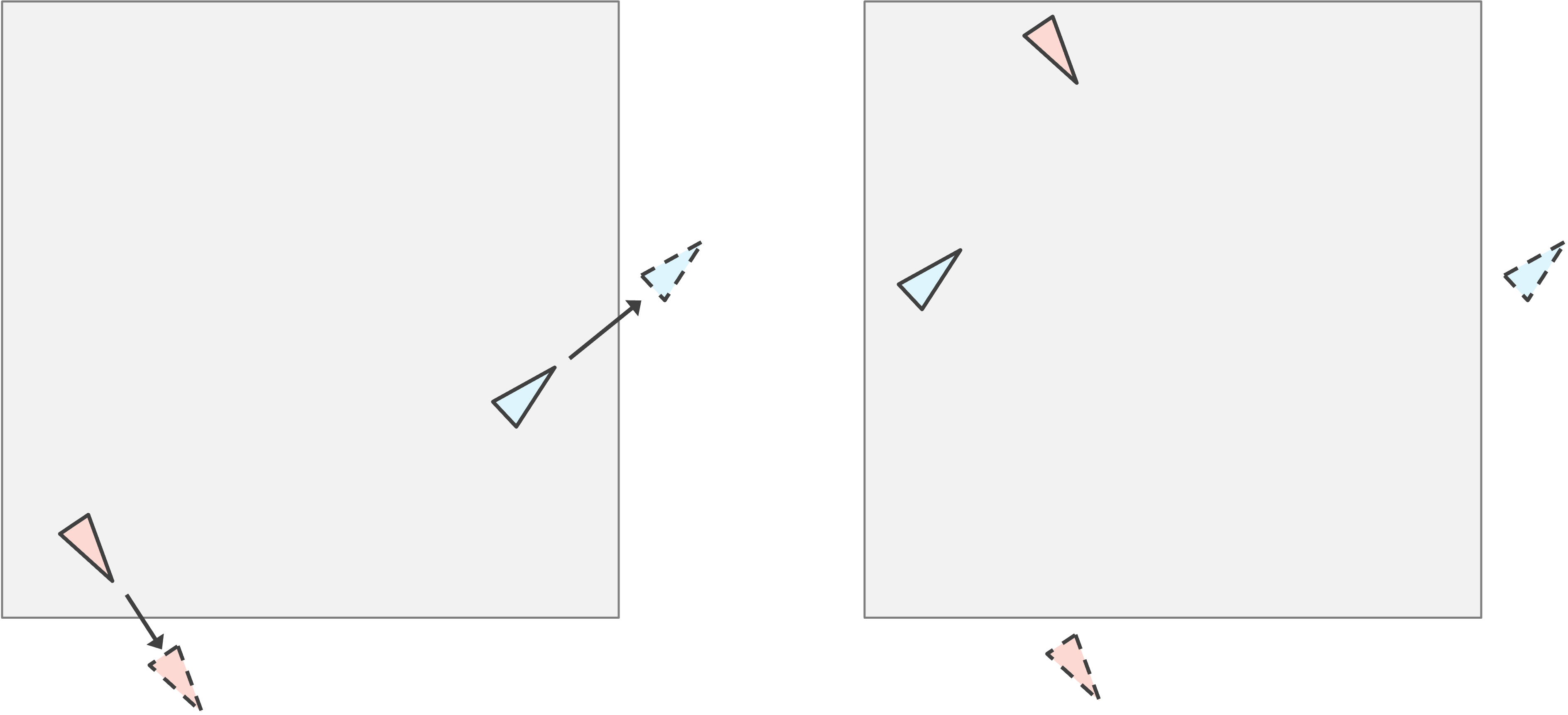
Boids fly on a torus

When building a gravity simulator, we assumed that the celestial bodies were confined to a square “universe” object because the force of gravity is an attractive one that keeps bodies from flying away.

In the boids simulation, we would either need an enormous board, or else a flock of boids would quickly migrate off the edge of the board en route to Florida, never to be heard from again. To ensure that boids are always visible, we will conceive that the left and right edge of the board are joined together, and the top and bottom edge of the board are joined together, so that when a boid flies off one side of the board, it reappears on the other side, as illustrated in the figure below.

This animation trick was first popularized by the video game “Asteroids” in 1979, shown below. For the nerds out there, both our boids simulation and Asteroids render objects on a “torus”, or a donut.

An object-oriented representation of the boid system

The following object-oriented design is provided in the starter code; you should not edit it.

As we used a Universe object to represent a system of heavenly bodies, we will use a Sky object to represent a system of boids at a single time point. A Sky object contains a width parameter and a list of Boid objects, as well as the following system parameters:

• proximity: the threshold distance within which boids interact;
• separation_factor, alignment_factor, and cohesion_factor: the constants c_separation, c_alignment, and c_cohesion introduced previously;
• max_boid_speed: the maximum speed any boid is allowed to travel.

class Sky:
    def __init__(
        self,
        width: float = 0.0,
        boids: list[Boid] = None,
        max_boid_speed: float = 0.0,
        proximity: float = 0.0,
        separation_factor: float = 0.0,
        alignment_factor: float = 0.0,
        cohesion_factor: float = 0.0,
    ):
        self.width = width
        self.boids = boids if boids is not None else []
        self.max_boid_speed = max_boid_speed
        self.proximity = proximity
        self.separation_factor = separation_factor
        self.alignment_factor = alignment_factor
        self.cohesion_factor = cohesion_factor

A Boid object contains the position, velocity, and acceleration of the boid, all represented as OrderedPair objects.

class Boid:
    def __init__(self, position: OrderedPair, velocity: OrderedPair, acceleration: OrderedPair):
        self.position = position
        self.velocity = velocity
        self.acceleration = acceleration

Finally, an OrderedPair object contains x- and y-components.

class OrderedPair:
    def __init__(self, x: float = 0.0, y: float = 0.0):
        self.x = x
        self.y = y

Required functions

You will implement ten functions. The highest-level function is simulate_boids(), which takes a Sky object initial_sky, a number of generations num_gens, and a time interval time_step, and returns a list of num_gens + 1 total Sky objects:

def simulate_boids(initial_sky: Sky, num_gens: int, time_step: float) -> list[Sky]:

This function calls update_sky(), which in turn calls three functions to update acceleration, velocity, and position:

def update_sky(current_sky: Sky, time_step: float) -> Sky:
def update_acceleration(current_sky: Sky, i: int) -> OrderedPair:
def update_velocity(
    b: Boid,
    old_acceleration: OrderedPair,
    max_boid_speed: float,
    time_step: float,
) -> OrderedPair:
def update_position(
    b: Boid,
    old_acceleration: OrderedPair,
    old_velocity: OrderedPair,
    sky_width: float,
    time_step: float,
) -> OrderedPair:

These functions rely on four additional functions you will also implement:

def net_acceleration_due_to_separation(current_sky: Sky, i: int) -> OrderedPair:
def net_acceleration_due_to_alignment(current_sky: Sky, i: int) -> OrderedPair:
def net_acceleration_due_to_cohesion(current_sky: Sky, i: int) -> OrderedPair:
def limit_speed(vel: OrderedPair, max_speed: float) -> OrderedPair:
def sum_vectors(*vectors: OrderedPair) -> OrderedPair:

The full function hierarchy is shown below.

simulate_boids
└── update_sky
    ├── update_acceleration
    │   ├── net_acceleration_due_to_separation
    │   ├── net_acceleration_due_to_alignment
    │   └── net_acceleration_due_to_cohesion
    ├── update_velocity
    │   └── limit_speed
    └── update_position
        └── (torus wrapping)
└── (utility used throughout) sum_vectors, distance

Running your program

Your program should be runnable from the command line as follows (use python instead of python3 on Windows):

python3 main.py num_boids sky_width initial_speed max_boid_speed num_gens proximity separation_factor alignment_factor cohesion_factor time_step canvas_width image_frequency

Your program should first generate a Sky object containing num_boids boids, each with an initial speed of initial_speed in a randomly chosen direction, a random position, and zero initial acceleration. It should then simulate the system for num_gens + 1 generations, capping any boid’s speed at max_boid_speed after each time step.

Rendering an animation

After producing the simulation, your program should generate an animated MP4 visualizing the boids on a canvas of canvas_width × canvas_width pixels, drawing only the i-th Sky object when i is divisible by image_frequency.

Here are some suggested parameters that produce a beautiful simulation (it may take a few minutes to run — please share if you find other nice parameters!):

python3 main.py 200 5000 1.0 2.0 8000 200 1.5 1.0 0.02 1.0 2000 20

Utility functions

Boids can only travel so fast, so we implement the following function to cap their speed. Recall that if a boid’s speed s exceeds maxBoidSpeed, we rescale both velocity components by maxBoidSpeed/s.

Computing the net acceleration

The next three functions each take a Sky object and the index i of a boid within it. They return an OrderedPair representing the net acceleration on current_sky.boids[i] due to each of the three boid forces, computed as the average force exerted by all nearby boids (those within current_sky.proximity). A boid does not exert a force on itself. If no other boids are within range, the acceleration is zero.

Updating boid state

Now that we have the three individual acceleration contributions, we can combine them and propagate the simulation forward in time.

Using the dynamics equations introduced previously, we can now update a boid’s velocity given its old and new acceleration values. Recall that if a boid’s updated speed exceeds maxBoidSpeed, its velocity must be rescaled.

Similarly, we can update a boid’s position using the dynamics equations. Remember that boids wrap around the edges of the sky — when a boid flies off one side of the board, it reappears on the other.

Simulating the boids

We are now ready to assemble the full simulation. Note that when updating a sky, all boids must be updated simultaneously — you should compute the new acceleration, velocity, and position of every boid using the current sky before writing any updated values back.